Why are my waveforms not detrending?

Well, I’m back again…

I’m developing a section plot, but my waveforms for the plot are not detrending and I can’t work out why. I have a lot of debugging traps in the code to switch on and off as required to try to work out where the problem is, so the code looks a bit messy no doubt.

I think I’m doing everything the same as I normally do, and I’ve tried other methods such as detrending the final stream rather than each trace, but all the results are the same. I’ve also tried all options for the detrending method.

Ultimately I want to have the section plot as a subplot beside a map, but I’ve commented that code out for now (as it has it’s own problems) while I concentrate on the detrending.

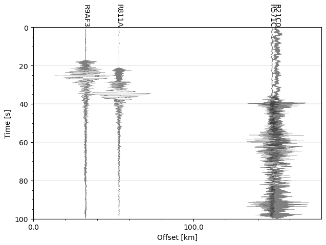
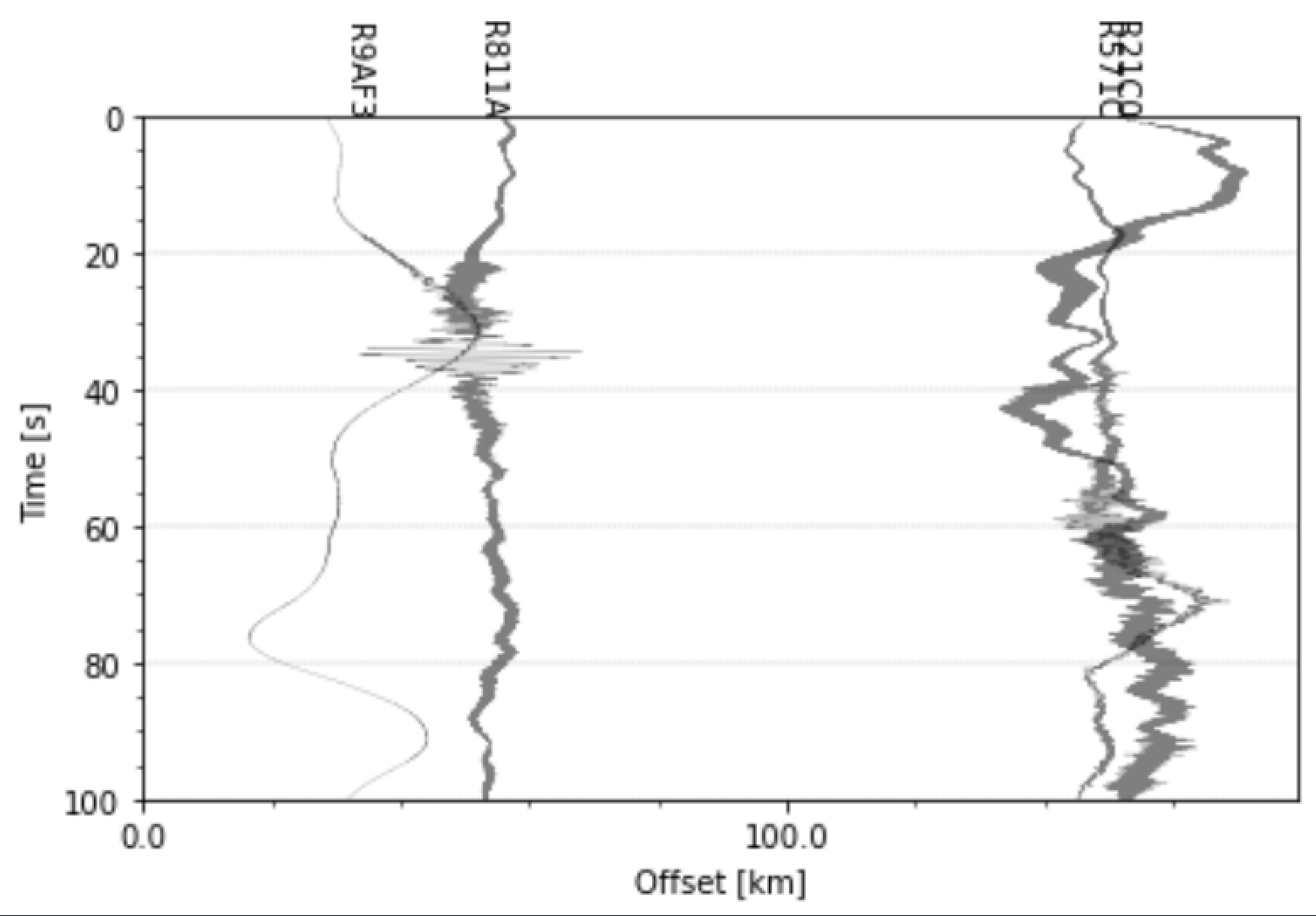
Here’s what my section plot currently looks like:

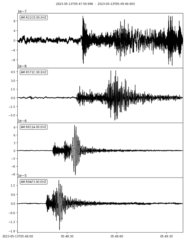
And this is the stream plot I’m producing as a debugging trap just before the section plot, showing the detrending is not working there either:

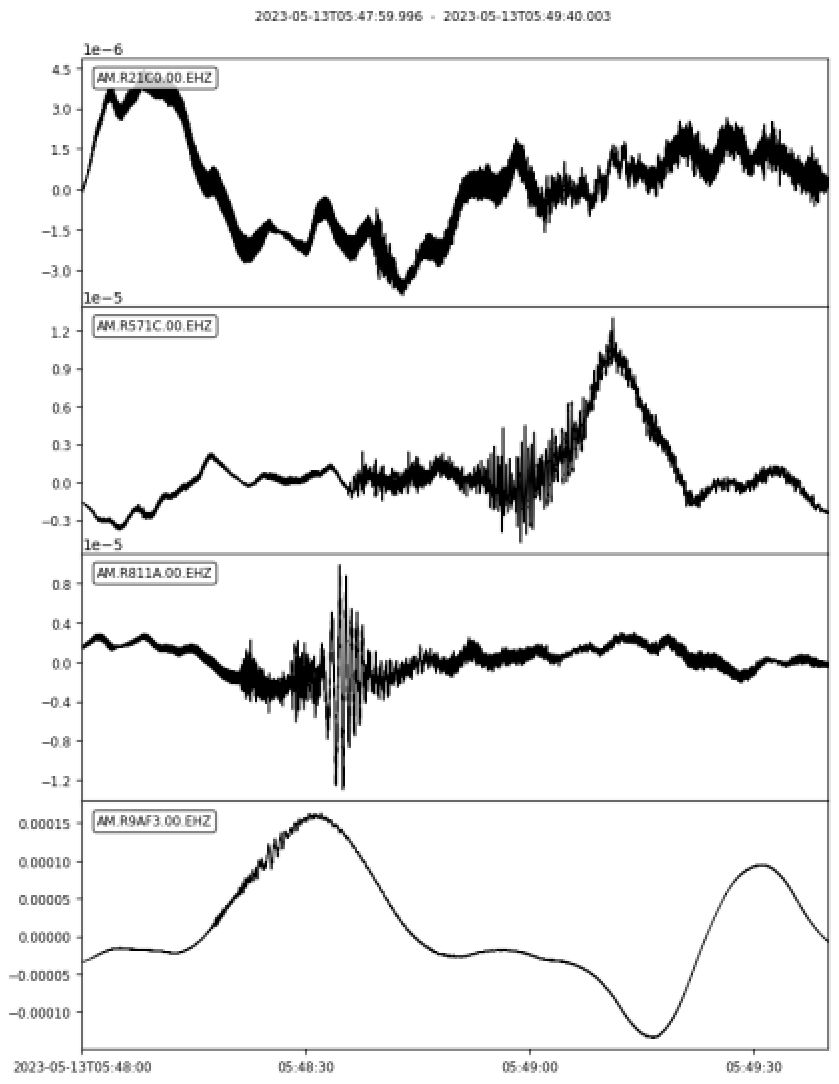
My plan is to have the local shakes in a list so I can simply comment out those I do not want to show if they don’t have data - mainly for small local quakes.

This is my code ATM:


# -*- coding: utf-8 -*-
"""
Created on Sun May 21 12:22:53 2023

@author: al72
"""

from obspy.clients.fdsn import Client
from obspy.core import UTCDateTime, Stream
#from obspy.signal import filter
import matplotlib.pyplot as plt
#from matplotlib.ticker import AutoMinorLocator
#import numpy as np
#from obspy.taup import TauPyModel
#import math
#import cartopy.crs as ccrs
#import cartopy.feature as cfeature
from matplotlib.transforms import blended_transform_factory
from obspy.geodetics import gps2dist_azimuth

rs = Client('https://data.raspberryshake.org/')

def stationList(sl):
    sl += ['R21C0']
    sl += ['R811A']
    sl += ['R9AF3']
    sl += ['R571C']
    #sl += ['R6D2A']
    #sl += ['RF35D']
    #sl += ['R7AF5']
    #sl += ['R3756']
    #sl += ['R6707']
    #sl += ['RB18D']
    #print(sl)
    return sl
    
def freqFilter(ft):
    # bandpass filter - select to suit system noise and range of quake
    #ft = "'bandpass', freqmin=0.1, freqmax=0.8"
    #ft = "'bandpass', freqmin=0.3, freqmax=0.8"
    #ft = "'bandpass', freqmin=0.5, freqmax=2"
    #ft = "'bandpass', freqmin=0.7, freqmax=2"       #distant quake
    #ft = "'bandpass', freqmin=0.7, freqmax=3"
    #ft = "'bandpass', freqmin=0.7, freqmax=4"
    #ft = "'bandpass', freqmin=0.7, freqmax=6"
    #ft = "'bandpass', freqmin=0.7, freqmax=8"
    #ft = "'bandpass', freqmin=0.7, freqmax=10"
    #ft = "'bandpass', freqmin=1, freqmax=20"
    #ft = "'bandpass', freqmin=3, freqmax=20"        #use for local quakes
    #ft = [0.1, 0.1, 0.8, 0.9]
    #ft = [0.3, 0.3, 0.8, 0.9]
    #ft = [0.5, 0.5, 2, 2.1]
    ft = [0.7, 0.7, 2, 2.1]       #distant quake
    #ft = [0.7, 0.7, 3, 3.1]
    #ft = [0.7, 0.7, 4, 4.1]
    #ft = [0.7, 0.7, 6, 6.1]
    #ft = [0.7, 0.7, 8, 8.1]
    #ft = [1, 1, 10, 10.1]
    #ft = [1, 1, 20, 20.1]
    #ft = [3, 3, 20, 20.1]        #use for local quakes
    print(ft)
    return ft
 
def buildStream(strm):
    n = len(slist)
    print(n)
    #stream = Stream()
    for i in range(0, n):
        inv = rs.get_stations(network='AM', station=slist[i], level='RESP')  # get the instrument response
        #print(inv[0])
        
        #read each epoch to find the one that's active for the event
        k=0
        while True:
            sta = inv[0][k]         #station metadata
            if sta.is_active(time=eventTime):
                break
            k += 1
        latS = sta.latitude     #active station latitude
        lonS = sta.longitude     #active station longitude
        #eleS = sta.elevation     #active station elevation
        print(slist[i], latS, lonS)
        print(sta)
        trace = rs.get_waveforms('AM', station=slist[i], location = "00", channel = 'EHZ', starttime = start, endtime = end)
        trace.merge(method=0, fill_value='latest')         #fill in any gaps in the data to prevent a crash
        trace.detrend(type='demean')                       #detrend the data
        #trace.filter(filt)
        tr1 = trace.remove_response(inventory=inv,zero_mean=True,pre_filt=filt,output='VEL',water_level=60, plot=False) # convert to Vel
        #print(tr[0])
        tr1[0].stats.distance = gps2dist_azimuth(latS, lonS, latE, lonE)[0]
        strm += tr1
    #strm.remove_response
    #strm.detrend(type='demean')
    strm.plot(method='full', equal_scale=False)
    return strm
    
eventTime = UTCDateTime(2023, 5, 13, 5, 48, 00) # (YYYY, m, d, H, M, S) **** Enter data****
latE = -32.4                           # quake latitude + N -S **** Enter data****
lonE = 150.0                        # quake longitude + E - W **** Enter data****
depth = 1                             # quake depth, km **** Enter data****
mag = 1                              # quake magnitude **** Enter data****
eventID = 'unknown'               # ID for the event **** Enter data****
locE = "Mudgeeish, NSW, Australia"                # location name **** Enter data****
#print(eventID)

slist = []
#filt = ""
filt = []
stationList(slist)
freqFilter(filt)
#print(slist)
print(filt)

#set up the plot
delay = 0
duration = 100
start = eventTime + delay
end = start + duration

st = Stream()
buildStream(st)
print(st)
#for t in st:
    #t.stats.distance = gps2dist_azimuth(t.stats.station.latitude, t.stats.station.longitude, latE, lonE)[0]

fig = plt.figure()
st.plot(type='section', plot_dx=100e3, recordstart=delay, recordlength=duration, equal_scale=False, time_down=True, linewidth=.25, grid_linewidth=.25, show=False, fig=fig)

# Plot customization: Add station labels to offset axis
ax = fig.axes[0]
transform = blended_transform_factory(ax.transData, ax.transAxes)
for tr in st:
    ax.text(tr.stats.distance / 1e3, 1.0, tr.stats.station, rotation=270, va="bottom", ha="center", transform=transform, zorder=10)
    print(tr.stats.distance)
"""    
fig = plt.figure(figsize=(20,14), dpi=150)       # set to page size in inches
ax1 = fig.add_subplot(1,2,1)
#ax2 = fig.add_subplot(1,2,2)
st.plot(type='section', plot_dx=20e3, recordlength=100, time_down=True, linewidth=.25, grid_linewidth=.25, show=False, fig=ax1)
# Plot customization: Add station labels to offset axis
ax = ax1.axes
transform = blended_transform_factory(ax.transData, ax.transAxes)
for t in st:
    ax.text(t.stats.distance / 1e3, 1.0, t.stats.station, rotation=270,
            va="bottom", ha="center", transform=transform, zorder=10)
"""
plt.show()

Whatever the problem is, I’m not seeing it ATM. Probably (hopefully) something very simple.

Thanks,

Al.

1 Like

Hello Al,

I admit, this thing was baffling, it never happened to me while I worked with similar code. It appears that the key to address the problem was in the water_level option. Lowering it from the original 60 to this value

tr1 = trace.remove_response(inventory=inv,zero_mean=True,pre_filt=filt,output='VEL',water_level=0.001, plot=False) # convert to Vel

manages to produce the following:

image

It would be interesting to understand in full why this was happening, but this edit should get you on the road, as they say.

1 Like

Wow! That’s a bit different. I didn’t think to play with the water level, as it works OK in all my other code. I was thinking there would be something really trivial and obscure that I’d got wrong and wasn’t seeing. Weird indeed.

Well done Stormchaser, and Thanks!

When I get a chance I might have to write some code experiment with the water level to better understand it.

Al.

2 Likes

Same here, I even substituted the code I use for my scripts and the result was the same, so there must be something somewhere else that we are not seeing.

In any case, this small adjustment should do the job, and the more stations you add to the plot, the more you can verify this.

No trouble at all, you’re welcome! Looking forward to your final product sheeny.

1 Like

G’Day Stormchaser,

I think I’ve solved why the waveforms were not detrending!

The way I was using a function to assign the filter corners resulted in the filter array being converted to a string. This doesn’t generate an error, however!

I twigged to it when I noticed the waveforms didn’t seem to change when I changed the filter.

So for now I’ve abandoned the function to assign the filter corners and I’ve put the filter code back into the main procedure, and now I find the waveforms detrend properly and the water_level can go back to 60.

Here’s the current code:


# -*- coding: utf-8 -*-
"""
Created on Sun May 21 12:22:53 2023

@author: al72
"""

from obspy.clients.fdsn import Client
from obspy.core import UTCDateTime, Stream
#from obspy.signal import filter
import matplotlib.pyplot as plt
#from matplotlib.ticker import AutoMinorLocator
#import numpy as np
from obspy.taup import TauPyModel
#import math
import cartopy.crs as ccrs
import cartopy.feature as cfeature
from matplotlib.transforms import blended_transform_factory
from obspy.geodetics import gps2dist_azimuth, kilometers2degrees, degrees2kilometers

rs = Client('https://data.raspberryshake.org/')

def stationList(sl):
    sl += ['R21C0']
    sl += ['R811A']
    sl += ['R9AF3']
    sl += ['R571C']
    #sl += ['R6D2A']
    #sl += ['RF35D']
    sl += ['R7AF5']
    #sl += ['R3756']
    #sl += ['R6707']
    #sl += ['RB18D']
    #sl += ['R9A9D']
    #sl += ['RCF6A']
    #print(sl)
    return sl
    
def buildStream(strm):
    n = len(slist)
    #print(n)
    tr1 = []
    #strm = []
    for i in range(0, n):
        inv = rs.get_stations(network='AM', station=slist[i], level='RESP')  # get the instrument response
        #print(inv[0])
        
        #read each epoch to find the one that's active for the event
        k=0
        while True:
            sta = inv[0][k]         #station metadata
            if sta.is_active(time=eventTime):
                break
            k += 1
        latS = sta.latitude     #active station latitude
        lonS = sta.longitude     #active station longitude
        #eleS = sta.elevation     #active station elevation
        #print(slist[i], latS, lonS)
        print(sta)
        trace = rs.get_waveforms('AM', station=slist[i], location = "00", channel = 'EHZ', starttime = start, endtime = end)
        trace.merge(method=0, fill_value='latest')         #fill in any gaps in the data to prevent a crash
        trace.detrend(type='demean')                       #detrend the data
        tr1 = trace.remove_response(inventory=inv,zero_mean=True,pre_filt=ft,output='VEL',water_level=60, plot=False) # convert to Vel
        tr1[0].stats.distance = gps2dist_azimuth(latS, lonS, latE, lonE)[0]
        tr1[0].stats.latitude = latS
        tr1[0].stats.longitude = lonS
        tr1[0].stats.colour = colours[i]
        strm += tr1
    #strm.plot(method='full', equal_scale=False)
    return strm

def k2d(x):
    return kilometers2degrees(x)

def d2k(x):
    return degrees2kilometers(x)

places = [['Oberon', -33.704922, 149.862900, 2],
          ['Bathurst', -33.419281, 149.577499, 4],
          ['Lithgow', -33.480930, 150.157410, 4],
          ['Mudgee', -32.590439, 149.588684, 4],
          ['Orange', -33.283333, 149.100006, 4],
          ['Sydney', -33.868820, 151.209290, 6],
          ['Newcastle', -32.926670, 151.780014, 6],
          ['Coonabarabran', -31.273911, 149.277420, 4],
          ['Gulgong', -32.362492, 149.532104, 2],
          ['Narrabri', -30.325060, 149.782974, 4],
          ['Muswellbrook', -32.265221, 150.888184, 4],
          #['Tamworth', -31.092749, 150.932037, 4],
          #['Boorowa', -34.437340, 148.717972, 2],
          #['Cowra,', -33.828144, 148.677856, 4],
          #['Goulburn', -34.754539, 149.717819, 4],
          #['Grafton', -29.690960, 152.932968, 4],
          #['Coffs Harbour', -30.296350, 153.115692, 4],
          #['Armidale', -30.512960, 151.669418, 4],
          #['Brisbane', -27.469770, 153.025131, 6]
          ]
    
eventTime = UTCDateTime(2023, 5, 13, 5, 48, 12) # (YYYY, m, d, H, M, S) **** Enter data****
latE = -32.33                           # quake latitude + N -S **** Enter data****
lonE = 149.93                        # quake longitude + E - W **** Enter data****
depth = 0                             # quake depth, km **** Enter data****
mag = 1                              # quake magnitude **** Enter data****
eventID = 'unknown'               # ID for the event **** Enter data****
locE = "Mudgeeish, NSW, Australia"                # location name **** Enter data****

slist = []
stationList(slist)
# bandpass filter - select to suit system noise and range of quake
#ft = [0.1, 0.1, 0.8, 0.9]
#ft = [0.3, 0.3, 0.8, 0.9]
#ft = [0.5, 0.5, 2, 2.1]
#ft = [0.7, 0.7, 2, 2.1]       #distant quake
#ft = [0.7, 0.7, 3, 3.1]
#ft = [0.7, 0.7, 4, 4.1]
#ft = [0.7, 0.7, 6, 6.1]
#ft = [0.7, 0.7, 8, 8.1]
#ft = [1, 1, 10, 10.1]
ft = [1, 1, 20, 20.1]
#ft = [3, 3, 20, 20.1]        #use for local quakesprint(filt[1], filt[2])
colours = ['r', 'b', 'g', 'k', 'c', 'm', 'purple', 'orange', 'gold', 'midnightblue']
plist = ('P', 'S')
#print(slist)
#print(ft)

#set up the plot
delay = 0
duration = 60
start = eventTime + delay
end = start + duration

st = Stream()
buildStream(st)
#print(st)

#set up the figure
fig = plt.figure(figsize=(20,14), dpi=100)       # set to page size in inches

#build the section plot
ax1 = fig.add_subplot(1,2,1)
st.plot(type='section', plot_dx=50e3, recordlength=duration, time_down=True, linewidth=.25, grid_linewidth=.25, show=False, fig=fig)

# Plot customization: Add station labels to offset axis
ax = ax1.axes
transform = blended_transform_factory(ax.transData, ax.transAxes)
for t in st:
    ax.text(t.stats.distance / 1e3, 1.0, t.stats.station, rotation=90,
            va="bottom", ha="center", color=t.stats.colour, transform=transform, zorder=10)

#setup secondary x axis
secax_x1 = ax1.secondary_xaxis('top', functions = (k2d, d2k))

#plot arrivals times
model = TauPyModel(model="iasp91")
#ax = plot_travel_times(source_depth=1, ax=ax, fig=fig, max_degrees=1.6, phase_list=['P', 'S'])

for t in st:
    arr = model.get_travel_times(depth, k2d(t.stats.distance/1000), phase_list=plist)
    n = len(arr)
    #print(arr)
    for i in range(0,n):
        ax.plot(t.stats.distance/1000, arr[i].time, marker='_', markersize=50, color = colours[plist.index(arr[i].name)], alpha=0.3)
        ax.text(t.stats.distance/1000+8, arr[i].time, arr[i].name, color=colours[plist.index(arr[i].name)], alpha=0.3)
                
"""  
arr = model.get_travel_times(depth, 0.8, phase_list=plist)
n = len(arr)
for i in range(0,n):
    ax.plot([0,d2k(0.8)], [0, arr[i].time], linestyle = '--', linewidth=0.5, color=colours[plist.index(arr[i].name)], alpha=0.3)
"""
#plot the map
ax2 = fig.add_subplot(1,2,2, projection=ccrs.PlateCarree())
mt = -30
mb = -35
ml = 148
mr = 152
ax2.set_extent([ml,mr,mt,mb], crs=ccrs.PlateCarree())
#ax2.coastlines(resolution='110m')
#ax2.stock_img()
# Create a features
states_provinces = cfeature.NaturalEarthFeature(
    category='cultural',
    name='admin_1_states_provinces_lines',
    scale='50m',
    facecolor='none')
ax2.add_feature(cfeature.LAND)
ax2.add_feature(cfeature.OCEAN)
ax2.add_feature(cfeature.COASTLINE)
ax2.add_feature(states_provinces, edgecolor='gray')
ax2.add_feature(cfeature.LAKES, alpha=0.5)
ax2.add_feature(cfeature.RIVERS)
ax2.gridlines(draw_labels=True)
#plot event/earthquake position on map
ax2.plot(lonE, latE,
     color='yellow', marker='*', markersize=20, markeredgecolor='black',
     transform=ccrs.Geodetic(),
     )
ax2.text(lonE+0.1, latE-0.05, "("+str(latE)+", "+str(lonE)+")\n"+eventTime.strftime('%d/%m/%y %H:%M:%S UTC'))

#plot station positions on map
for tr in st:
    ax2.plot(tr.stats.longitude, tr.stats.latitude,
             color=tr.stats.colour, marker='H', markersize=12, markeredgecolor='black',
             transform=ccrs.Geodetic(),
             )

#plot places
for pl in places:
    ax2.plot(pl[2], pl[1], color='k', marker='o', markersize=pl[3], markeredgecolor='k', transform=ccrs.Geodetic(), label=pl[0])
    ax2.text(pl[2], pl[1]-0.1, pl[0], horizontalalignment='center', transform=ccrs.Geodetic())

#add notes to map
ax2.text((ml+mr)/2, mt-0.2, 'M'+str(mag)+' Earthquake at '+locE, ha='center')
ax2.text((ml+mr)/2, mt-0.3, 'Depth = '+str(depth)+' km. ID = '+eventID, ha='center')
ax2.text((ml+mr)/2, mt-0.4, 'Filter = '+str(ft[1])+' to '+str(ft[2])+' Hz.', ha='center')


plt.subplots_adjust(wspace=0.1)

plt.show()

2 Likes

Good day to you sheeny,

Ah! That was the cause then; it’s good that you managed to isolate and fix it, so now you can continue your project without having to think about it anymore.

Thank you for the code as usual; I’m sure others will find it interesting as I do!

1 Like