Is it possible to add corner frequencies to the RSUDP plot?
1 Like
Hello Wanderingjeep, and welcome to our community!
Yes, it is possible to add them. However, to do so, you will have to manually edit your local RSUDP installation files so that the plotting module will display what you have in mind.
You can find more information on how the modules work together here: rsudp 1.1.1 — rsudp documentation. In particular, I think you may have to edit the c_plot sub-consumer (rsudp.c_plot (plot data) — rsudp documentation).
As I think this could be very interesting for the rest of the community, any progress that you want to share is more than welcome!
Thanks for the hint about where to get this done, Stormchaser. I have always wanted to apply a filter to RSUDP
I added one line to c_plot.py (it took a few tries to get the right place and syntax ![]() ).
).
I added this line. self.stream.filter(‘bandpass’, freqmin=.3, freqmax=8, corners=4)
It was added to mainloop:
def mainloop(self, i, u):
	'''
	The main loop in the :py:func:`rsudp.c_plot.Plot.run`.

	:param int i: number of plot events without clearing the linecache
	:param int u: queue blocking counter
	:return: number of plot events without clearing the linecache and queue blocking counter
	:rtype: int, int
	'''
	if i > 10:
		linecache.clearcache()
		i = 0
	else:
		i += 1
	self.stream = rs.copy(self.stream)	# essential, otherwise the stream has a memory leak
	self.raw = rs.copy(self.raw)		# and could eventually crash the machine
	self.deconvolve()
	self.stream.filter('bandpass', freqmin=.3, freqmax=8, corners=4)
	self.update_plot()
	if u >= 0:				# avoiding a matplotlib broadcast error
		self.figloop()

	if self.save:
		# save the plot
		if (self.save_timer > self.save[0][0]):
			self._eventsave()
	u = 0
	time.sleep(0.005)		# wait a ms to see if another packet will arrive
	sys.stdout.flush()
	return i, u
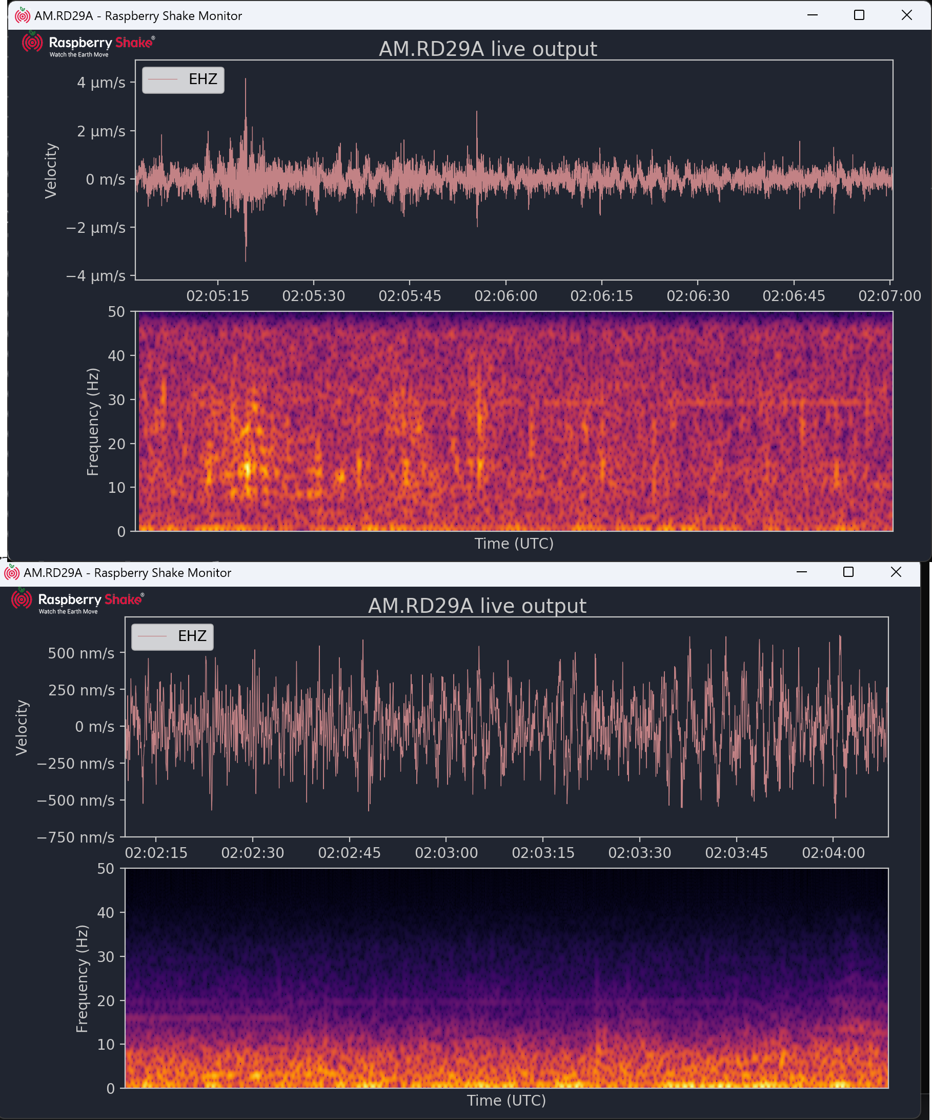
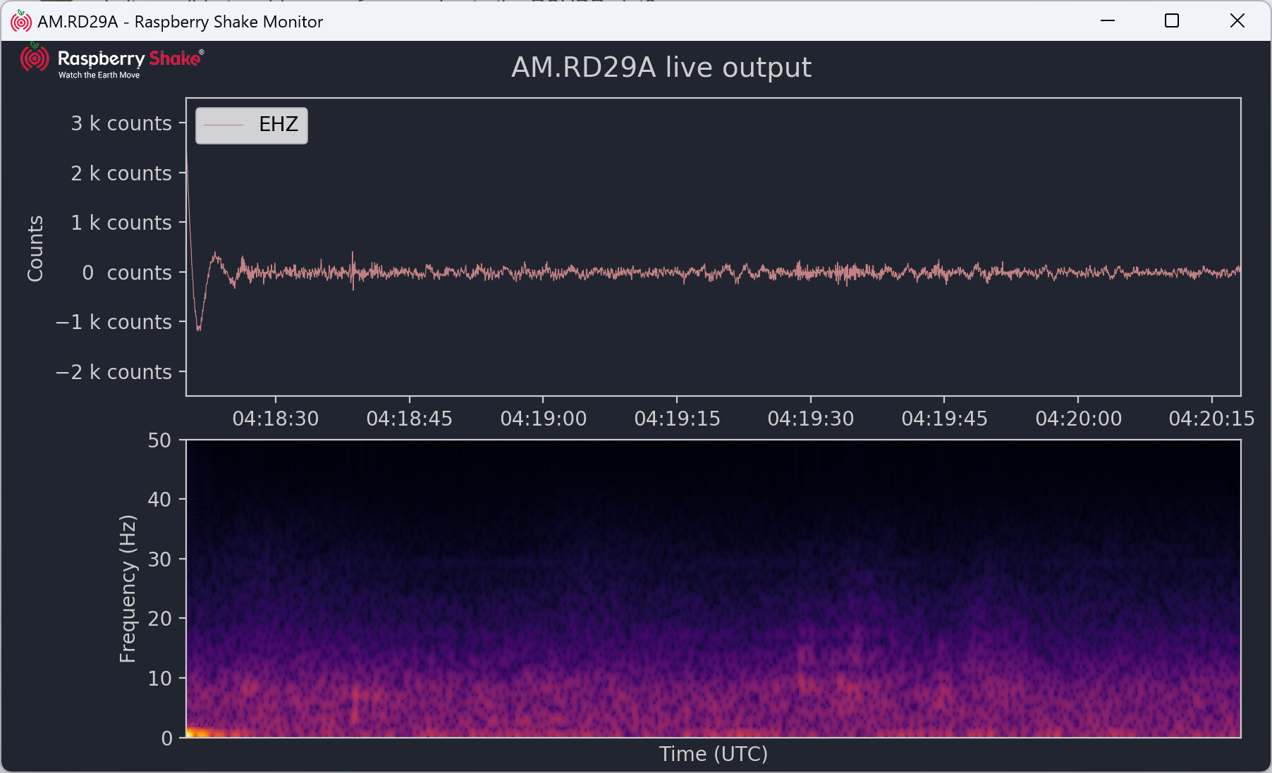
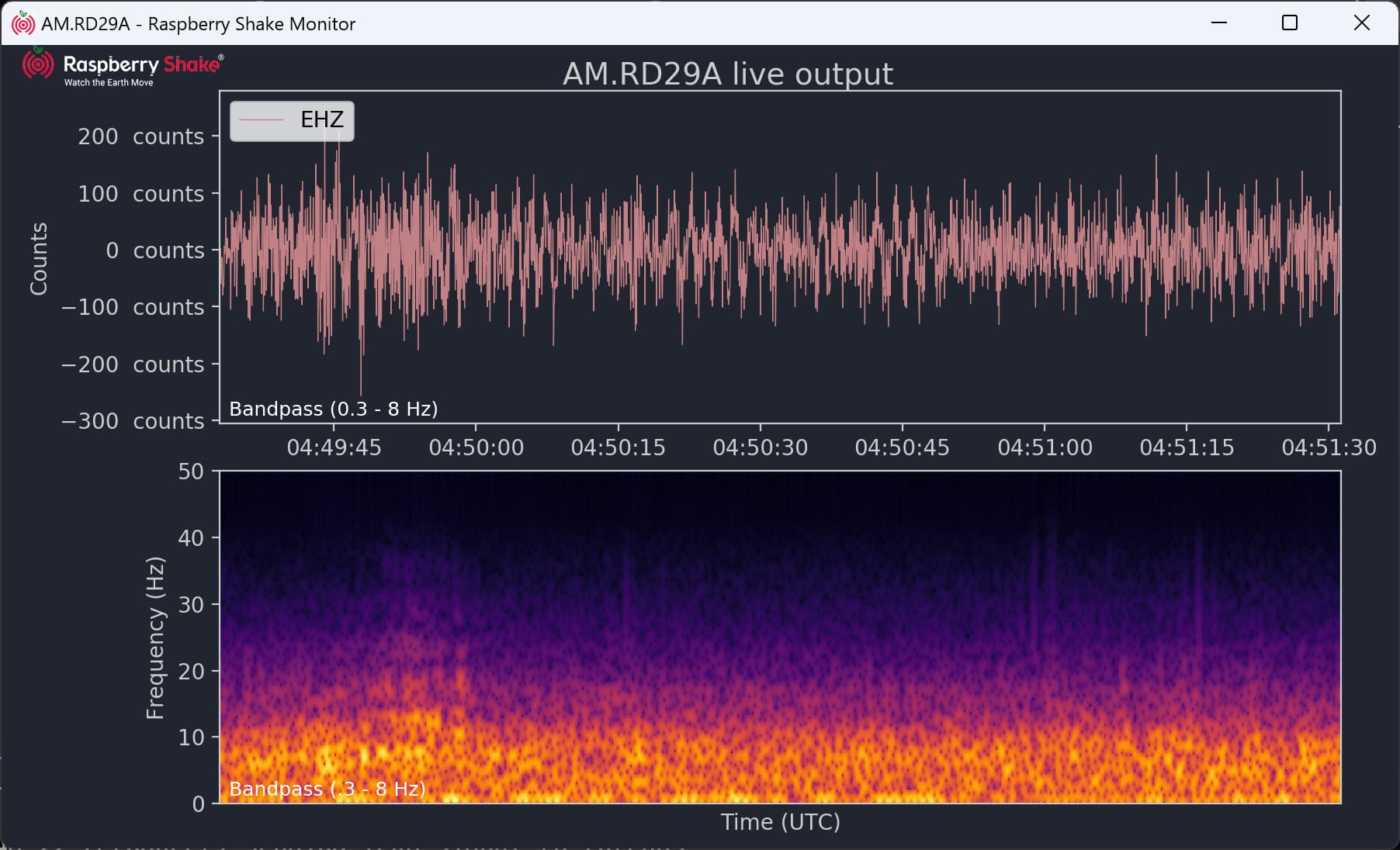
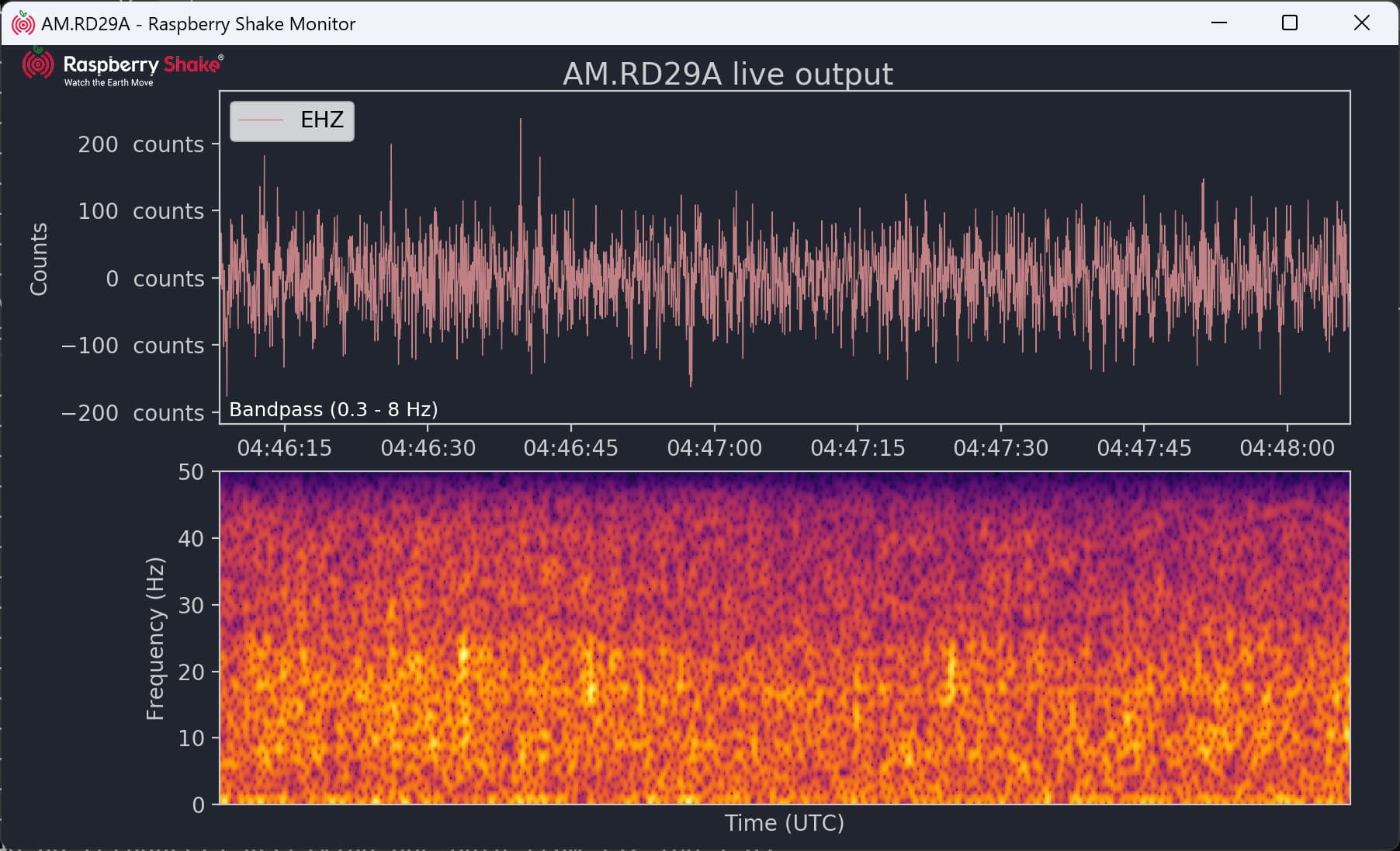
Results before and after
Notes:
- If the new filter line is added before self.deconvolve() line, no filtering takes place
- I have only tested with one channel
- Ideally, I would like to filter the waveform only and leave the spectrogram unfiltered. However, I need to spend more time to see if this is possible. I am not sure if I can pass around a filtered and non-filtered stream
- If I set “deconvolve”: false in settings, I get a large wave stuck on the left-hand side that does not clear. So, my solution does not work with counts
So, it’s not perfect, but it does work. I am sure there are better ways to get it done.
–Steve
RD29A - Chino Hills, Ca
2 Likes
Always welcome Steve, and great update! Thank you so much for sharing it with the community.
(I am going to try this too ![]() )
)
And I agree, possible further steps could be:
- turning on/off the filtering option for the trace/spectrogram from the
.jsonconfig file - making variables out of the filtering frequencies in the config file, so that they can be edited in an easier way
However, already having a filtered trace/spectrogram could be useful for many (myself included) who do not live in or close to earthquake-active areas and only see events in the lower frequency ranges.
HI Stormchaser,
I agree. Making the filter a toggle and parameterizing the filter frequencies are the correct next steps. Removing hard coding is always good.
Good news. I have split filtering working now. A filter is applied to the waveform and the spectrogram remains unfiltered. It took a good amount of trial and error as I learned the flow of rsudp.
I ended up making 6 more changes in addition to the one previously mentioned to filter both the waveform and spectrogram. The changes are in 3 sections of c_plot.py. Look for the ‘# SBC:’ comments. The changes made were to create an unfiltered copy of the stream object and have the spectrogram plot use the unfiltered data.
Sections changed:
- super().init()
- def _update_specgram(self, i, mean):
- def mainloop(self, i, u):
super().__init__()
		self.sender = 'Plot'
		self.alive = True
		self.testing = testing
		self.alarm = False			# don't touch this
		self.alarm_reset = False	# don't touch this


		if MPL == False:
			sys.stdout.flush()
			sys.exit()
		if QT == False:
			printW('Running on %s machine, using Tk instead of Qt' % (platform.machine()), self.sender)

		self.queue = q
		self.master_queue = None	# careful with this, this goes directly to the master consumer. gets set by main thread.

		self.stream = rs.Stream()
		self.raw = rs.Stream()
		self.stream_uf = rs.Stream() # SBC: Initialize stream_uf
		self.stn = rs.stn
		self.net = rs.net


	def _update_specgram(self, i, mean):
		'''
		Updates the spectrogram and its labels.

		:param int i: the trace number
		:param float mean: the mean of data in the trace
		'''
		self.nfft1 = self._nearest_pow_2(self.sps)	# FFTs run much faster if the number of transforms is a power of 2
		self.nlap1 = self.nfft1 * self.per_lap
		if len(self.stream_uf[i].data) < self.nfft1: # SBC: Replaced Stream with Stream_uf
			self.nfft1 = 8
			self.nlap1 = 6
		sg = self.ax[i*self.mult+1].specgram(self.stream_uf[i].data-mean, # SBC: Replaced Stream with Stream_uf
					NFFT=self.nfft1, pad_to=int(self.nfft1*4), # previously self.sps*4),
					Fs=self.sps, noverlap=self.nlap1)[0]	# meat & potatoes
		self.ax[i*self.mult+1].clear()	# incredibly important, otherwise continues to draw over old images (gets exponentially slower)
		# cloogy way to shift the spectrogram to line up with the seismogram
		self.ax[i*self.mult+1].set_xlim(0.25,self.seconds-0.25)
		self.ax[i*self.mult+1].set_ylim(0,int(self.sps/2))
		# imshow to update the spectrogram
		self.ax[i*self.mult+1].imshow(np.flipud(sg**(1/float(10))), cmap='inferno',
				extent=(self.seconds-(1/(self.sps/float(len(self.stream_uf[i].data)))), # SBC: Replaced Stream with Stream_uf
						self.seconds,0,self.sps/2), aspect='auto')
		# some things that unfortunately can't be in the setup function:
		self.ax[i*self.mult+1].tick_params(axis='x', which='both',
				bottom=False, top=False, labelbottom=False)
		self.ax[i*self.mult+1].set_ylabel('Frequency (Hz)', color=self.fgcolor)
		self.ax[i*self.mult+1].set_xlabel('Time (UTC)', color=self.fgcolor)

	def mainloop(self, i, u):
		'''
		The main loop in the :py:func:`rsudp.c_plot.Plot.run`.

		:param int i: number of plot events without clearing the linecache
		:param int u: queue blocking counter
		:return: number of plot events without clearing the linecache and queue blocking counter
		:rtype: int, int
		'''
		if i > 10:
			linecache.clearcache()
			i = 0
		else:
			i += 1
		self.stream = rs.copy(self.stream) # essential, otherwise the stream has a memory leak
		self.raw = rs.copy(self.raw)		# and could eventually crash the machine
		self.stream_uf = rs.copy(self.stream_uf)  # SBC: Applied the same fix/patch as above to prevent memory leak
		self.deconvolve()
		self.stream_uf = self.stream.copy()  # SBC: Make an copy of the unfiltered Stream to be used with the Specto
		self.stream.filter('bandpass', freqmin=.3, freqmax=8, corners=4) # SBC: Filter for the waveform.
		self.update_plot()

		if u >= 0:				# avoiding a matplotlib broadcast error
			self.figloop()

		if self.save:
			# save the plot
			if (self.save_timer > self.save[0][0]):
				self._eventsave()
		u = 0
		time.sleep(0.005)		# wait a ms to see if another packet will arrive
		sys.stdout.flush()

		return i, u
Notes:
- Filter with counts still does not work.
- Only tested with one channel
- I am not a programmer. I have enough PHP and Python knowledge to plod through and figure things out. I am sure there are better and/or efficient ways to get it done
- So far, memory and CPU usage seems normal
–Steve
RD29A - Chino Hills, ca
2 Likes
A great result Steve!
I have tested your previous iteration, and it worked without issues on my side too, so I’m eager to try this one.
I’ll see if I can find a bit of time during the weekend to play with the .json parametrization and see what comes out.
1 Like
Hi Stormchaser,
Thanks for the feedback and good luck with the .json parametrization.
I did come up with a fix for the filter failing with counts. I ended up adding a single line. The line works when filtering both the waveform and spectrogram as well as waveform only.
Through a little googling, I found that the stream needs to be detrended when it has not been deconvolved before the filter is applied. I should have remembered this because I do the same thing in my infographic and my large graph on the live stream.
So, I added the same line of code I have been using: self.stream.detrend(type=‘demean’)
I added it just before the new filter line in the ‘mainloop’. As shown below:
    def mainloop(self, i, u):
        '''
        The main loop in the :py:func:`rsudp.c_plot.Plot.run`.

        :param int i: number of plot events without clearing the linecache
        :param int u: queue blocking counter
        :return: number of plot events without clearing the linecache and queue blocking counter
        :rtype: int, int
        '''
        if i > 10:
            linecache.clearcache()
            i = 0
        else:
            i += 1
        self.stream = rs.copy(self.stream)  # essential, otherwise the stream has a memory leak
        self.raw = rs.copy(self.raw)  # and could eventually crash the machine
        self.deconvolve()
        self.stream.detrend(type='demean') #SBC: Detrend added to fiter corectly when deconvolve = false (counts)
        self.stream.filter('bandpass', freqmin=.3, freqmax=8, corners=4) # SBC: Filter for the waveform.
        self.update_plot()
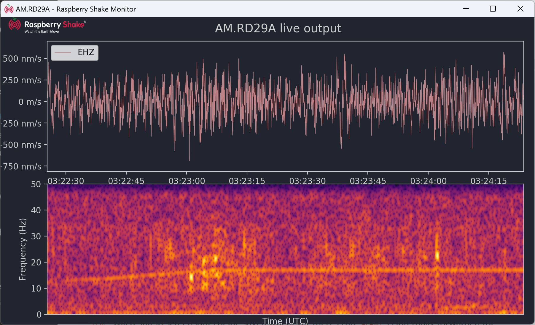
As I was testing the new line with counts, the 4.2 Lytle Creek occurred just 24mi/38km away. It provided a good test ![]() . This was using split filtering. The waveform was filtered and the spectrogram was not.
. This was using split filtering. The waveform was filtered and the spectrogram was not.
So, I think everything is in place and working to provide full (waveform and spectrogram) and split (waveform only) filtering. Next, as you pointed out, the changes need to be made to make the use of the filter(s) more user-friendly/configurable. Not everyone will want to go and start editing code ![]()
–Steve
RD29A - Chino Hills, Ca
Hi Stormchaser,
I could not help myself and I gave adding new .json settings a try :). It seems to be working as expected.
I am attaching the files I have updated: .json settings, c_plot.py, and client.py
I added the new filter settings to Plot. That seemed to make the most sense to me. The changes allow the waveform only, spectrogram only, or both to be filtered. I also added a label on the plots when filtering was enabled with the bandpass frequency values.
I commented my changes with SBC:. I think I got them all. Feel free to use any of my changes or make any necessary changes. I am taking a break now :). I have learned a lot and the updates work for my needs.
–Steve
RD29A - Chino Hills, Ca
rsudp_settings.json (1.6 KB)
c_plot.py (32.2 KB)
client.py (18.4 KB)
2 Likes
Hello Steve,
Apologies for my delay in replying, but I managed to sit down and take a look at this only this evening.
To summarize, fantastic work! I was working on a filtering protocol that went along with what you have down in your RSUDP installation, working mainly on c_plot.py, but I got “stuck” in a corner by using a different approach (trying to automate the waveform display with fewer variables in the .json).
Your approach, instead, is much more streamlined so I decided to scrap mine (that is, putting it on the back burner to come back to it at a later date) and test yours. I have RSUDP installed on my Win11 PC and on a Pi3B, it works perfectly fine on both. Even better, the filtered waveform (left the spectrogram as it is) allows me to extend the displayed trace to 120 seconds on the Pi, instead of the 60 I had before.
I also corrected this line on c_plot.py in the spectrogram portion of the code, which continued to retain the initial .3 - 8 Hz text and was not dynamically adapting to the user-updated .json data:
            self.ax[i * self.mult + 1].text(.008, .04, 'Bandpass (' + str(self.filter_highpass) + ' - ' + str(self.filter_lowpass) +' Hz)',
                                            fontsize=9,color='white', horizontalalignment='left',verticalalignment='center',
                                            transform = self.ax[i * self.mult + 1].transAxes)
After that, I also slightly edited the appearance of the Bandpass text in both plots, raising the y-value to 0.05 and changing the color from white to the basic one of the other texts:
                self.ax[i * self.mult].text(0.008, .05, 'Bandpass (' + str(self.filter_highpass) + ' - ' + str(self.filter_lowpass) +' Hz)',
                                            fontsize=9, color=self.fgcolor, ...
I think this is a fantastic step forward for RSUDP! Thank you so much for your continued passion and interest in this Steve!
Hi Stormchaser,
No problem with the delay. Thanks for the review and feedback. It’s good to hear it runs without issues or performance downgrades.
- Yes, I completely missed the swap of static to variables on the spectro label display.
- I like the new position and color update of the filter label. I kept changing y-position and was having a hard time settling on a value as I tried adding more channels or changing the size of the plot.
One more fix to add in. I found that I left a print statement in c_plot.py that I was using during my debugging. Remove the “print(axis)” below. This is the only change I made since uploading the files here.
def setup_plot(self):
    """
	Sets up the plot. Quite a lot of stuff happens in this function.
	Matplotlib backends are not threadsafe, so things are a little weird.
	See code comments for details.
	"""
    # instantiate a figure and set basic params
    self._init_plot()

    for i in range(self.num_chans):
        self._init_axes(i)

    for axis in self.ax:
        # set the rest of plot colors
        plt.setp(axis.spines.values(), color=self.fgcolor)
        plt.setp([axis.get_xticklines(), axis.get_yticklines()], color=self.fgcolor)
        print(axis)
Thanks @Wanderingjeep for posting the question and Stormchaser for pointing me in the right direction. It was an interesting and challenging process to get it all working. I am glad it turned out the way it did and others will be able to take advantage of the functionality.
–Steve
RD29A - Chino Hills Ca
2 Likes
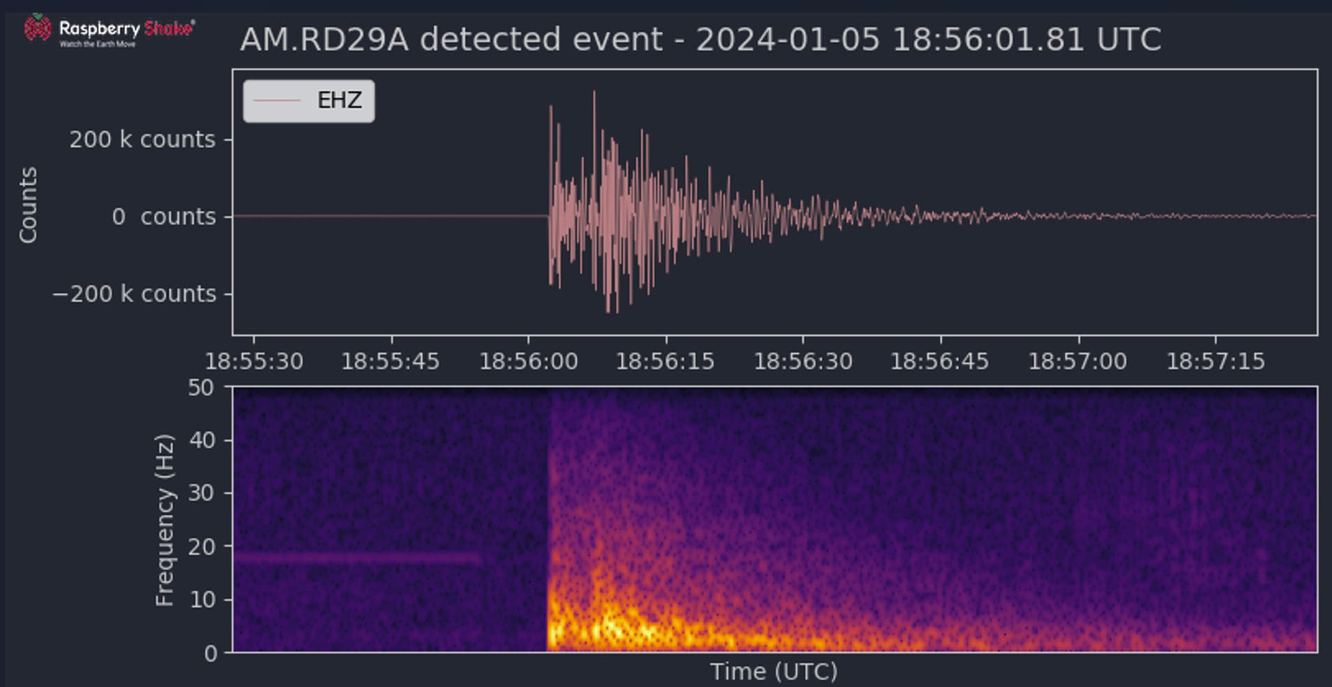
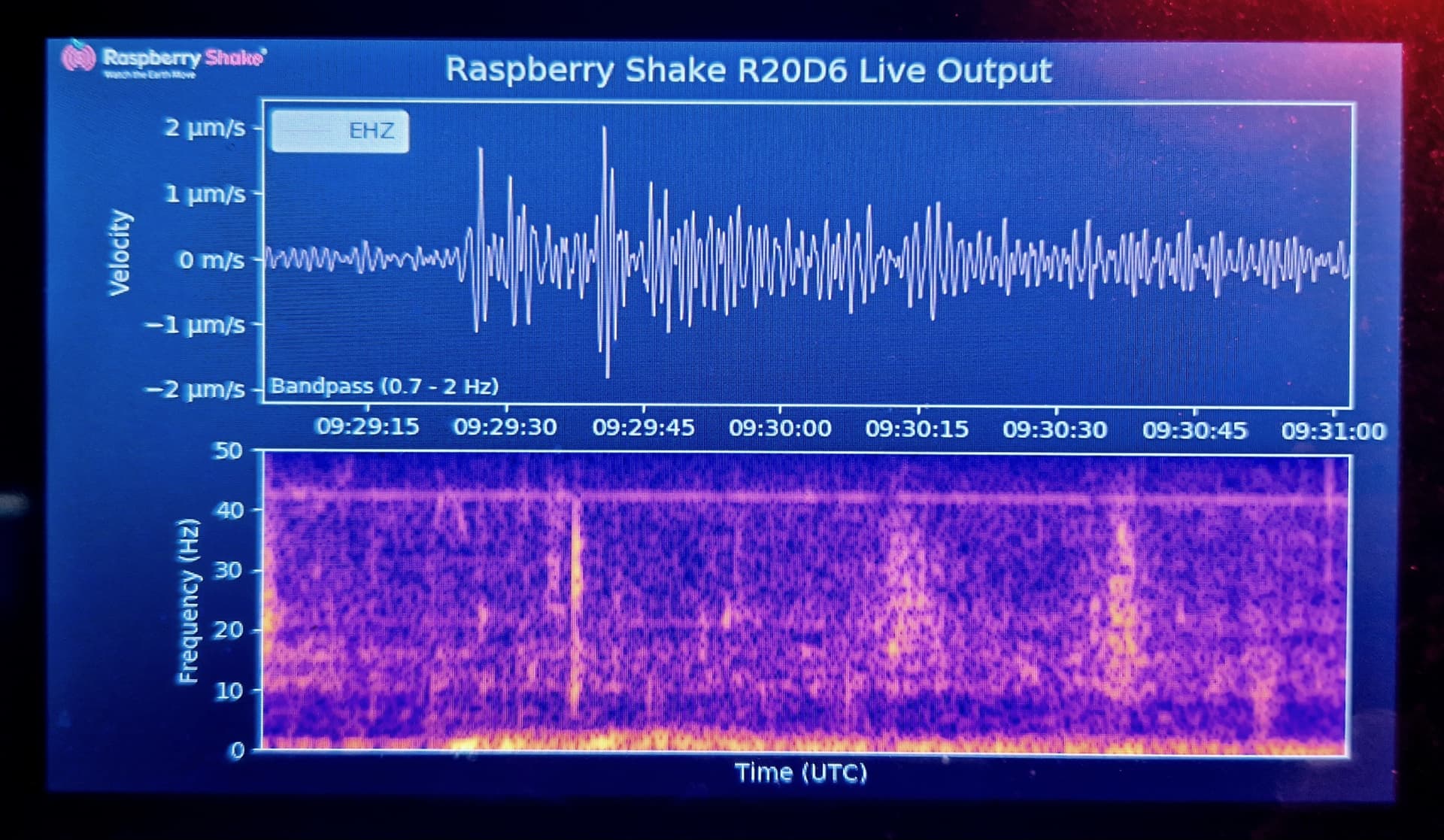
Working perfectly Steve! This is a quick snap of the P-wave from the M6.4 in Afghanistan as it reached my Shake here. Very clean plot with this filter.
1 Like
Hi Steve
!
I keep running into you😁 I had asked you about how you keep your stream running for so long. I asked it in the comments of your stream!
Bravo on your coding here. Wonderful! When i asked the question initially, I thought that maybe it was built in already and had no idea you and Stormchaser were going to modify the code. Then to my surprise, i stumbled across an email this morning that was a response to my original question and saw all the comments and code changes made!
.
Here is a link to my stream.

I downloaded your code and made the changes. You can see it in my stream now. Thank you!
2 Likes
Hello Wanderingjeep,
Fantastic work with your livestream; thank you for sharing it with us!
And, happy to help! Steve was the main driving force behind this, and I only applied some bits here and there.
Definitely hoping this topic will be able to help others that want to realize a similar project!
1 Like