RBoom versus a real SPL meter

[kpjamro]

I decided to start a new thread now that I have things working.

Summary - my results indicate that the RBoom readings are about 10 dB high versus an actual SPL meter. By implication, the pressure readings are high by about a factor of 4. Or I have made a mistake.

I made measurements on a passing airplane and produced SPL’s for two different frequency octaves using both RBoom and a calibrated microphone good to 10 Hz (umik-2).

Here is the summary:

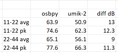
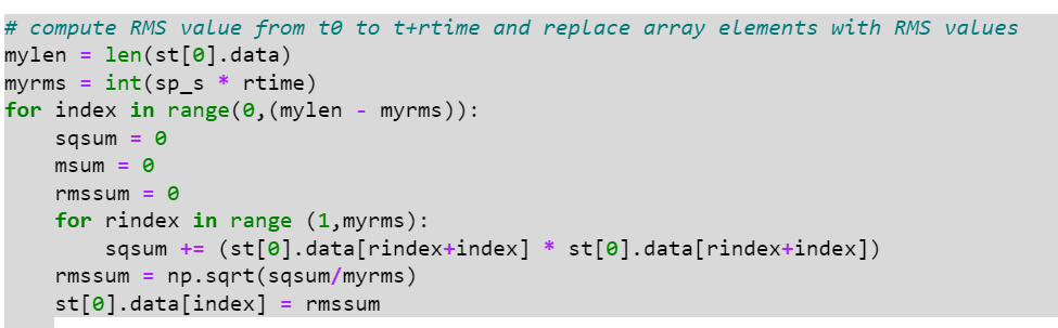
The routine for SPL using RBoom is from the example
https://manual.raspberryshake.org/developersCorner.html#converting-counts-to-pascal-to-decibel-using-obspy
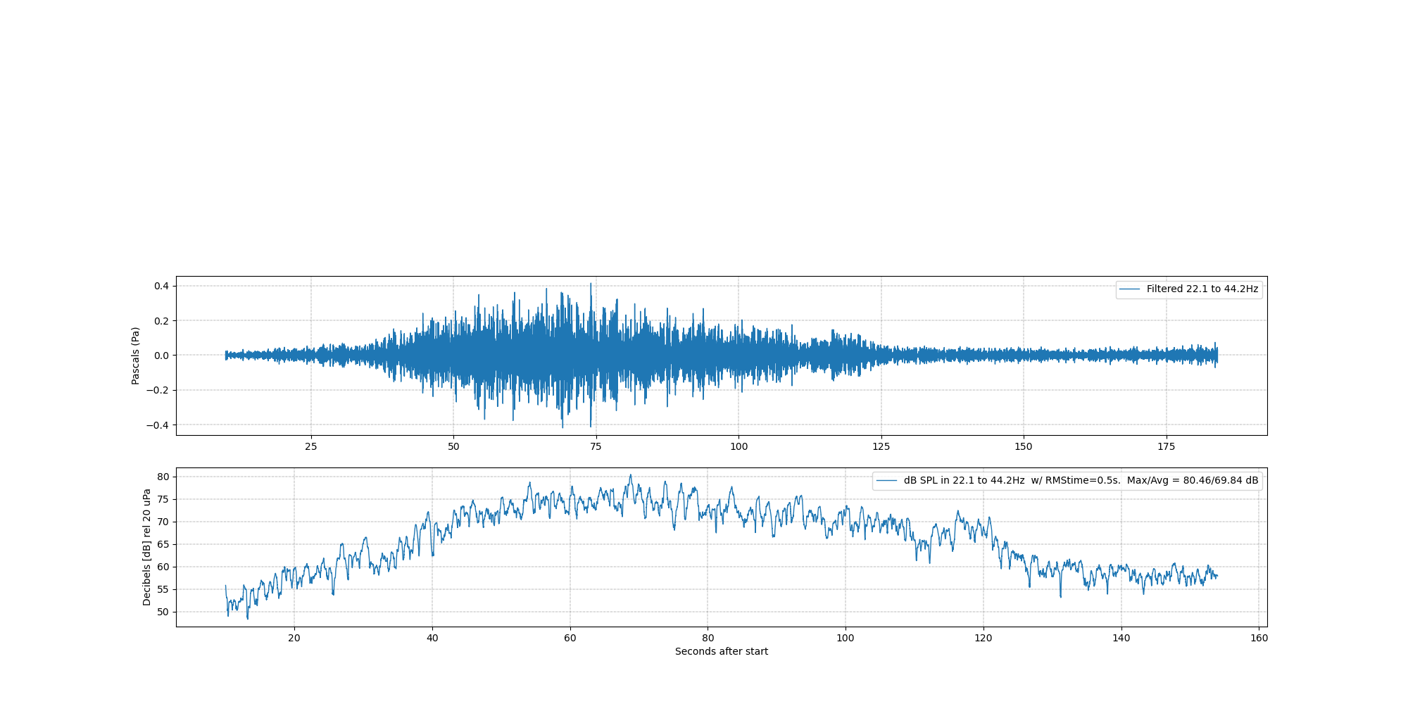
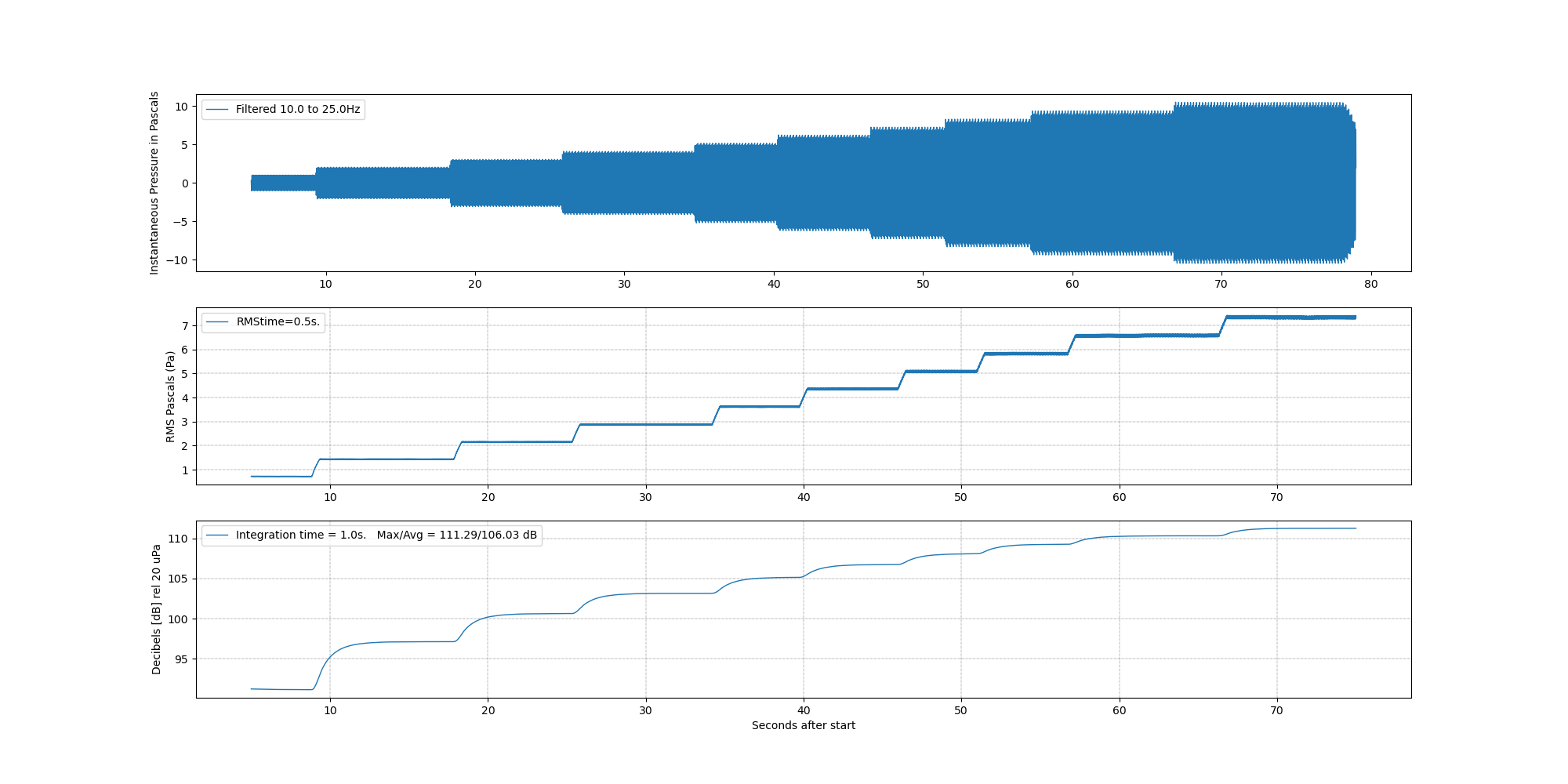
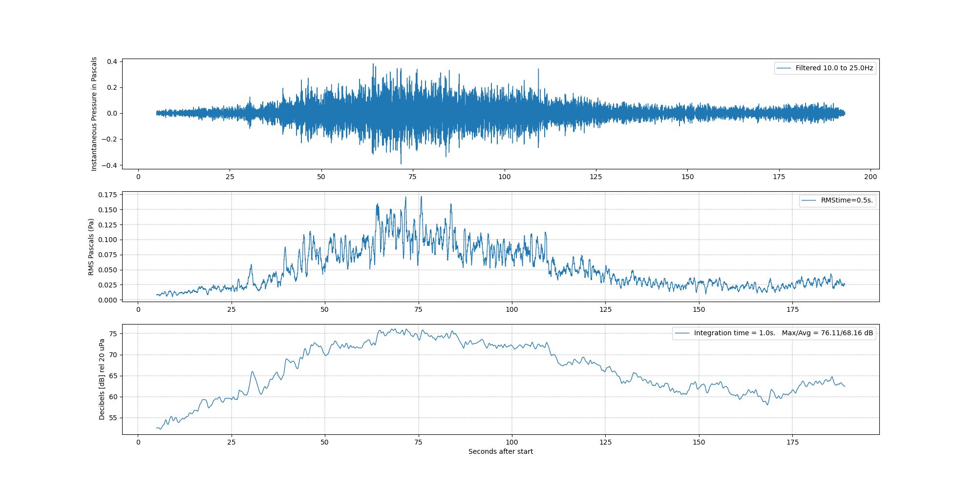
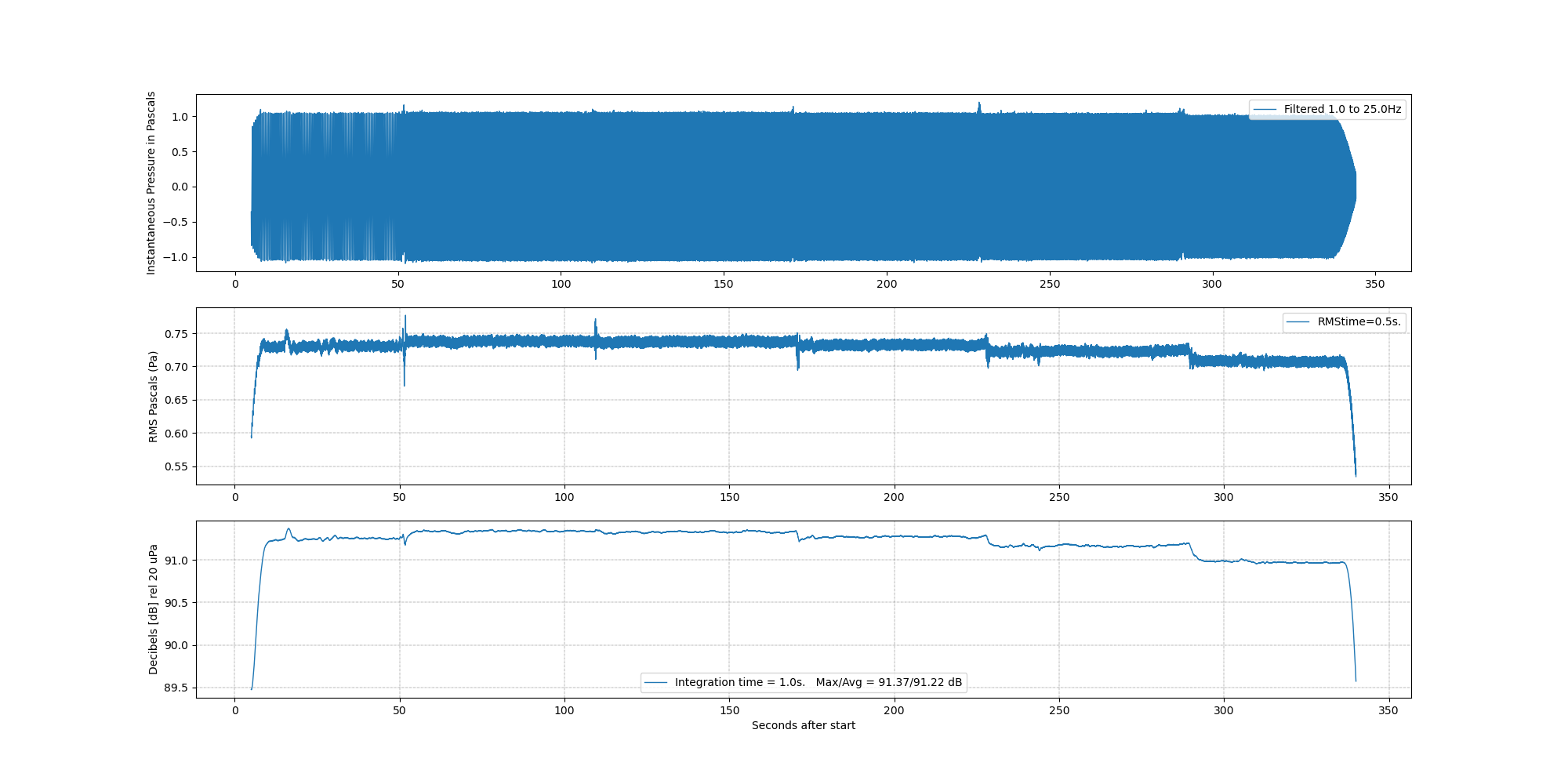
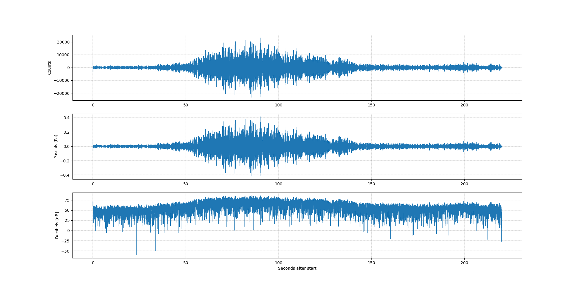
The code on the developers corner produces this graph with my airplane pass data

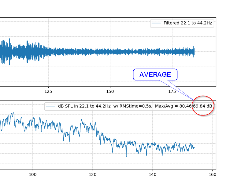
if I filter the data to extract 22-44 Hz, I get this:

Real SPL meters usually integrate the sound over 0.5 or 1.0 seconds.
In my code I did 0.5 second integration and it looks like this:

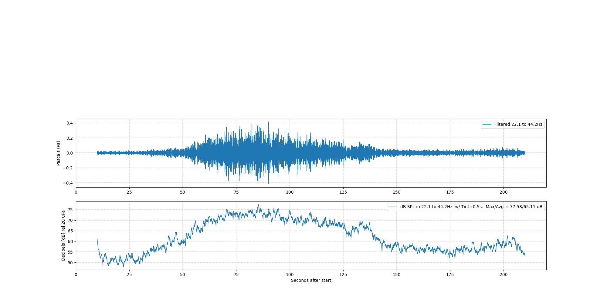
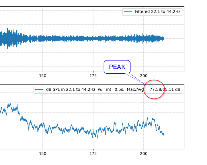
The octave band peak SPL comes out to be around 77 dB peak, down from 80+ in the unfiltered data.
But the result of the octave band is ~77 dB with, or without, the integration feature. With an airplane pass, what the integration mostly does is eliminate those occasional dips to --20 dB, when a single sample value happens to be near zero. If the sound is “impulsive” (gun shots or hammer blows?) then the integration would have a bigger effect.

What does a “real” SPL meter indicate? I used a calibrated USB microphone called UMIK-2. It comes with a calibration file that is compatible with a program called REW. With this combination, the readings should be within +/- 0.1 dB down to 10 Hz. I have checked it with a sound level calibrator that produces 94 dB at 1 kHz and I have, in turn, checked the calibrator against a real type-1 SPL meter - and the numbers are spot-on.

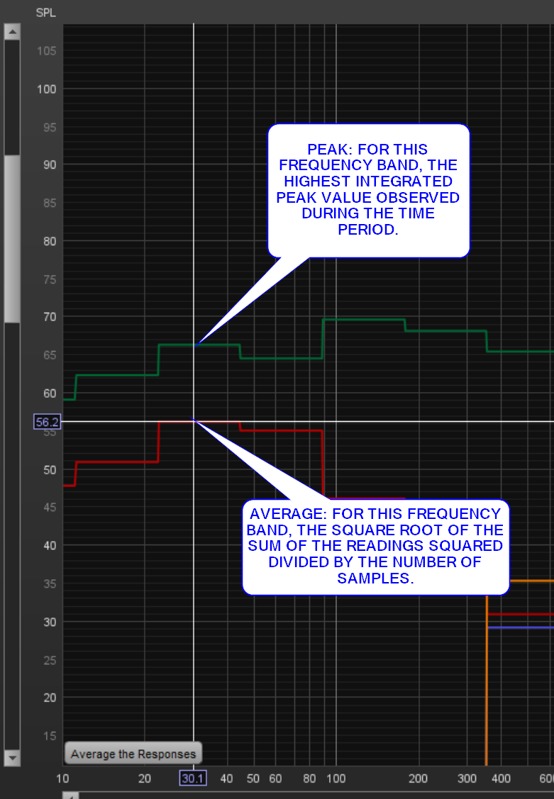
Here is the graphical output of REW:

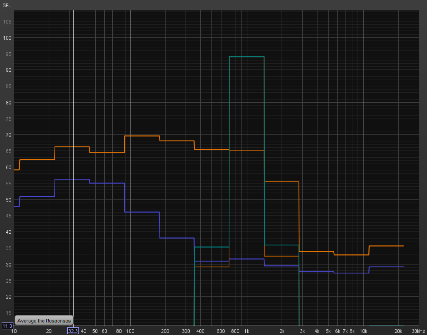
The green line is the calibration test: 94 dB at 1 kHz.
The orange and blue lines are the readings from my airplane recording showing the peak and the time-average values at each frequency octave band, respectively.

You can see the “real” SPL readings from the real meter are about 10 dB less than what RBoom indicates (when using the formula shown in the developer corner)…

Any ideas why?

(Disclosure - the input piping on my RB has a damped resonance around 25 Hz but I think the effect is less than 3 dB).

[Stormchaser]

Hello kpjamro,

Wow! This was a very interesting comparison with some great plots, overall well presented; thank you for taking the time to do this!

I am not sure of the reason behind the differences you have highlighted, which appear to be well calculated, so I leave the field open to anyone in the community who can add something to this topic.

[kpjamro]

Interesting article showing how you might calibrate a sensor like RB

infrasound-test.pdf (4.4 MB)

It’s in Appendix A.

You could use one of these:
specs_model60UHP.pdf (chaparralphysics.com)

and some more on testing these things:
Infrasound Sensor Models and Evaluation (columbia.edu)

[kpjamro]

More research indicates that you need to state exactly what quantity is being measured for your dB number. For compliance with municipal noise regulations it is almost always the RMS value of the sound wave. For example:

3.36 “RMS sound pressure” means the square root of the time averaged square of the sound pressure,
denoted Prms. ( Council Bluffs : Municipal Code (municipalcodeonline.com)

This sort of usage also has A-weighing or C-weightings applied to come up with a single number measurement. We are not applying weighting here.

Here is a nice discussion of the topic (in water, but the principle is the same);

Introduction to Signal Levels – Discovery of Sound in the Sea (dosits.org)

Based on the above, the example given on the RBoom developer web page is best described as “zero-to-peak dB”.

The REW “software SPL meter” applies exponential weighting to the peak graph and does RMS evaluation for the average reading. My guess is that REW uses the entire duration of the recording as the RMS basis. The analysis gives only 1 number for the RMS readings.

What do you suppose dB RMS would look like with RBOOM ?

[kpjamro]

This is what the RMS plot looks like (for one frequency band):

The max value actually went up by 3 dB - in hindsight, not surprising. The average went up a bit too.

The points in this graph are “moving” RMS values averaged over 0.5 seconds, or 50 samples.
This is similar to the moving average, except with elements squared/averaged/rooted.
The calculation is done in Pascals, then plotted in dB.

Here is the calc:

It’s interesting to see the slight changes to the curve and where the maximum value now occurs.
The Avg value of 69.84 dB is an average over the entire time period of the trace.

Tomorrow I will show the relationship between these graphs and the SPL meter functions of REW.

[kpjamro]

here is the summary:

From the measurement microphone and REW

Corresponding numbers from RBoom - one from integrated peaks graph the other from RMS graph.
(Note that the “RMStime” parameter pertains to the individual points on the RMS graph. The single printed average value is for the whole time period).

Integrated peaks:

RMS Average:

The bottom line is that the RBoom data comes out about 11 dB high on peak and 13 dB high on average (for the 22-44 Hz band),

I think the next step is to do another recording except to pull the tubing off the inlet piping manifold. This will eliminate the possibility that the inlet pipe array is somehow amplifying the sound (relative to how RBOOM was calibrated).

[Stormchaser]

I would say that this is an amazing analysis and presentation work kpjamro; thank you very much for sharing it with all the RS community!

I think I will take some days to read through it in full to understand all the steps you’ve taken.

[kpjamro]

Some time has passed and I have done more work.

The biggest discrepancy between RBoom and the SPL meter was the average value which, of course, is the main thing an SPL meter produces. I see now that I had a couple of errors in the way that was calculated. I fixed that. The other possibility is that sound pressure measurement itself was wrong, in one place or the other. In the spirit of trust-but-verify, I have now done a check of RBoom vs a Chaparral Physics Model 25 Infrasound Sensor and I have seen good agreement between the two. (I will post that separately).

I rearranged the process to compute RMS first and then do the time integration. I expect the RMS integration period will usually be less than the integration time. Setting these time constants is kind of undefined territory when you get down to single-digit frequencies. SPL readings are usually made for a specific acoustic band (1/3 octave for example). I can suggest that the RMS integration time be 1/F, where F is the lower limit of the octave band in question.

My test setup lets me produce a continuous signal of desired tone, or amplitude, which is a great help in figuring out things. With a single tone, the peak, the average and RMS are all the same.

Here is an example where a 15 Hz tone is stepped up in volume in 10 equal steps:

And here is the airplane pass from we have been talking about. The average value is much more reasonable now,

Lastly, here is a run where the amplitude is (nearly) constant but the frequency is varied in steps from 2 to 20 Hz.

The little “glitches” are from switching the signal generator frequency “on the fly”.

I will post the python code in the next reply.

[Stormchaser]

This is simply high-level and amazing kpjamro, thank you for sharing your extensive work with all of us in the community!

I will take care (also for personal interest) to bookmark and re-read this topic sometime in the future when I can dedicate myself to this in full, so that I can explore what my BOOM can do.

[kpjamro]

As promised, here is a writeup on my sound generator.
HOME MADE INFRASOUND SOURCE.pdf (629.0 KB)

[branden]

Thank you for independently confirming the published Sensitivity of the HDF channels of the RBOOM / RS&BOOM @kpjamro

branden