I was looking at:
https://manual.raspberryshake.org/developersCorner.html#converting-counts-to-pascal-to-decibel-using-obspy
and I have it running here.
I would like to compare RBOOM to a measurement microphone I have that is calibrated down to 10 Hz. I would use a 1/3 octave band around 15 Hz and maybe 30 Hz.
I think its easy to approximate the octave band filters by using the st.filter method with the right corner frequencies.
But the usual display of dB SPL involves an integration time for the data (exponential smoothing) rather than display of instantaneous values as in the script. Typical times are 0.5 and 1.0 seconds
I think I found a function to do this:
https://docs.obspy.org/packages/autogen/obspy.signal.util.smooth.html#obspy.signal.util.smooth
The “smoothie” parameter would be 50 or 100 values of 0.5 and 1.0 seconds.
But I lack the understanding of how to apply this to the signal in the python script referenced above.
Help.
1 Like
Hello kpjamro,
I have never used that function, so I cannot confirm if it is the one you are looking for. However, from the syntax, I think you have to “feed” the entire downloaded stream to the smoother function to get the output you are looking for.
In our case, the downloaded stream is st, so the smooth function should be stream_smooth = smooth(st, smoothie).
If not, the only other value that refers to the original signal is st[0].times(reftime=start) some lines below. But I don’t think this last is the correct one. You will have to make some trials and errors.
OK - I have had some success by operating on the actual elements of the trace, in place.
I used this:
# integration time
inttime = 0.5  #seconds
sps = 100  #sampling rate
f1 = 1/((sps + 1)*inttime) # fraction of each new sample
f2 = 1-f1
# smooth the data for the 3rd curve using exponential averaging
mylen = len(st[0].data)
for index in range(1,mylen):
    st[0].data[index] = f2*abs(st[0].data[index-1]) + f1*abs(st[0].data[index])
maxdb = st.max()
maxdb[0] = np.round(20*np.log10(abs(maxdb[0]/56000)/0.00002),2)
ax3.plot(st[0].times(reftime=start), 20*np.log10(abs(st[0].data/56000)/0.00002), lw=1)
note that you need to take the absolute value before trying to average.
But I have two questions:
-
Isn’t it necessary to remove the instrument response like with the RShake? I note that, in the example, you attach the response info, but never remove it. If you remove it, what output= do you specify? I tried DISP and VEL but they produce a really small output. Perhaps if you use one of these then the requirement to divide by 56000 goes away?
-
I need to do filtering as well. If I apply a bandpass filter, there is a big transient at the start which screws up the graphing scale and detection of max value. Using zerophase=True helps a bit, but not enough. This does not seem to be a problem with geophone data. What to do?
Thanks
1 Like
Hello kpjamro,
Good progress! In order:
- If I remember correctly, when writing that code, there was no option other than “displacement-velocity-acceleration” for the response removal step. They were naturally not applicable as we were analyzing pressure variation in Pascals, so I left it as you could see. You can try with the new
st.remove_response(output='DEF')
(obspy.core.trace.Trace.remove_response — ObsPy 1.4.0 documentation) and see if it produces results that are more reasonable to you. If so, then I will proceed to update the code on our manual.
- That artefact is something that I was never able to fully erase via simple filtering method(s) and, in the end, my solution was to simply “cut it out” from the final plotted waveform. Usually, the first 4-6 seconds were enough by using with this step before plotting:
st.trim(t1+6, t2)
If you find another viable method, please let us know!
Thank you.
1 Like
I will use the trim function for now.
There is a function called taper:
st.taper(max_percentage=0.05, type=“hann”)
But tapering to zero is minus infinite dB 
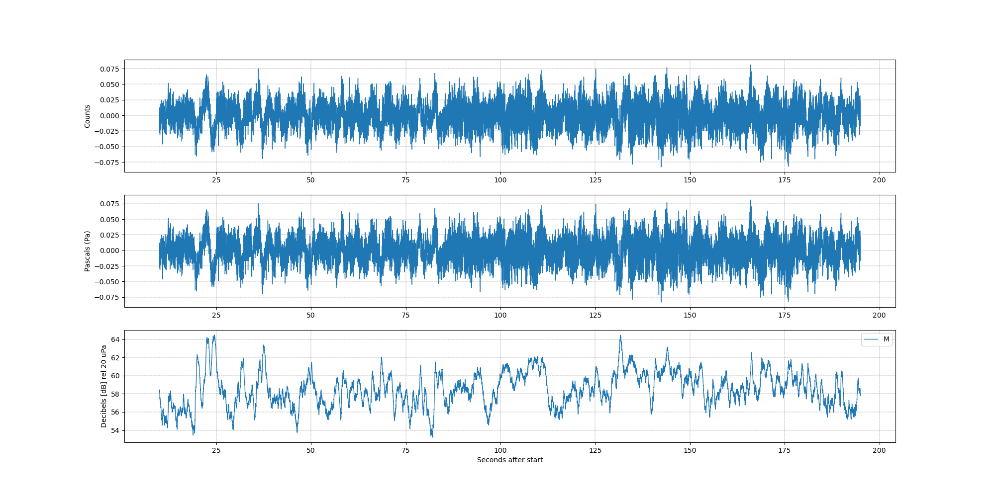
Here is what happens if you remove instrument response and use DEF.
(I removed the divide by 56000).
The counts and pascals become the same (because the raw value is now pascals instead of counts).
And you can see some very low frequency components. I don’t remember the filtering for this graph - it might have been Fmin = 0.1 Hz. You can see some waves in there approaching 10 seconds. Increase amplitude of the “bottom end” of the frequency range is what the instrument response does for you.
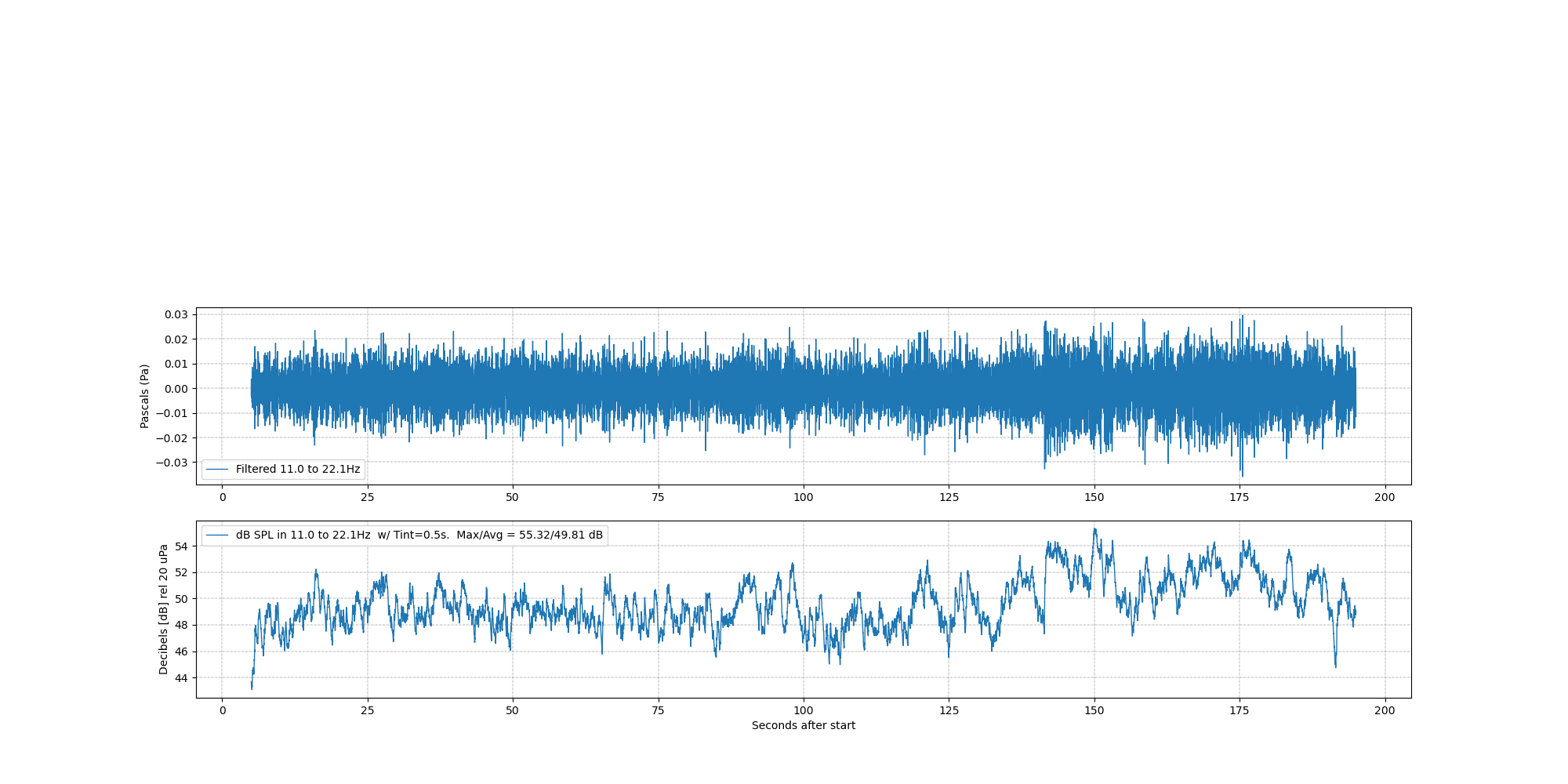
Next I put in frequency limits for “octave band 0” which is centered on 15.6 Hz and deleted the redundant trace:
Note that I added an average value. This is the value typically used for noise studies. It’s an average of the integrated peaks over the displayed time period.
I see that the default bandpass filter characteristic in Obspy is Butterworth which matches the flat-top shape in standard ANSI S1.11. Here is an old copy of that standard:
You could actually use bands as small as 1/3 octave. But, down below 30 Hz, perhaps that is a bit silly. Still, there might be reasons to focus on a narrow slice for a particular noise-making machine you want to single out and analyze.
I will have to figure out where to go from here, but the results look reasonable.
I will eventually drag my calibrated microphone and laptop out to where the RBOOM is and get some comparison data.
= = =
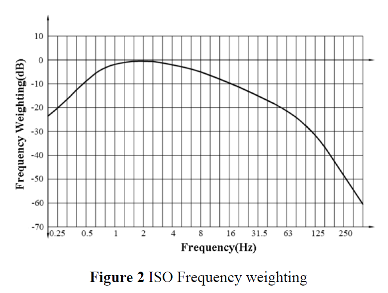
Stepping back to PPV … to calculate a single number for vibration in this (human sensitive) frequency range there is a weighting curve that should be applied:
It may be enough to filter it for 0.5-16 Hz and leave it at that.
stay tuned.
2 Likes
Will definitely stay tuned kpjamro, this is extremely interesting!
Thank you for your work and updates!