Raspbery Boom Self noise spec

[kpjamro]

I am trying to understand the noise spec a shown on the technical documents page.
This figure:

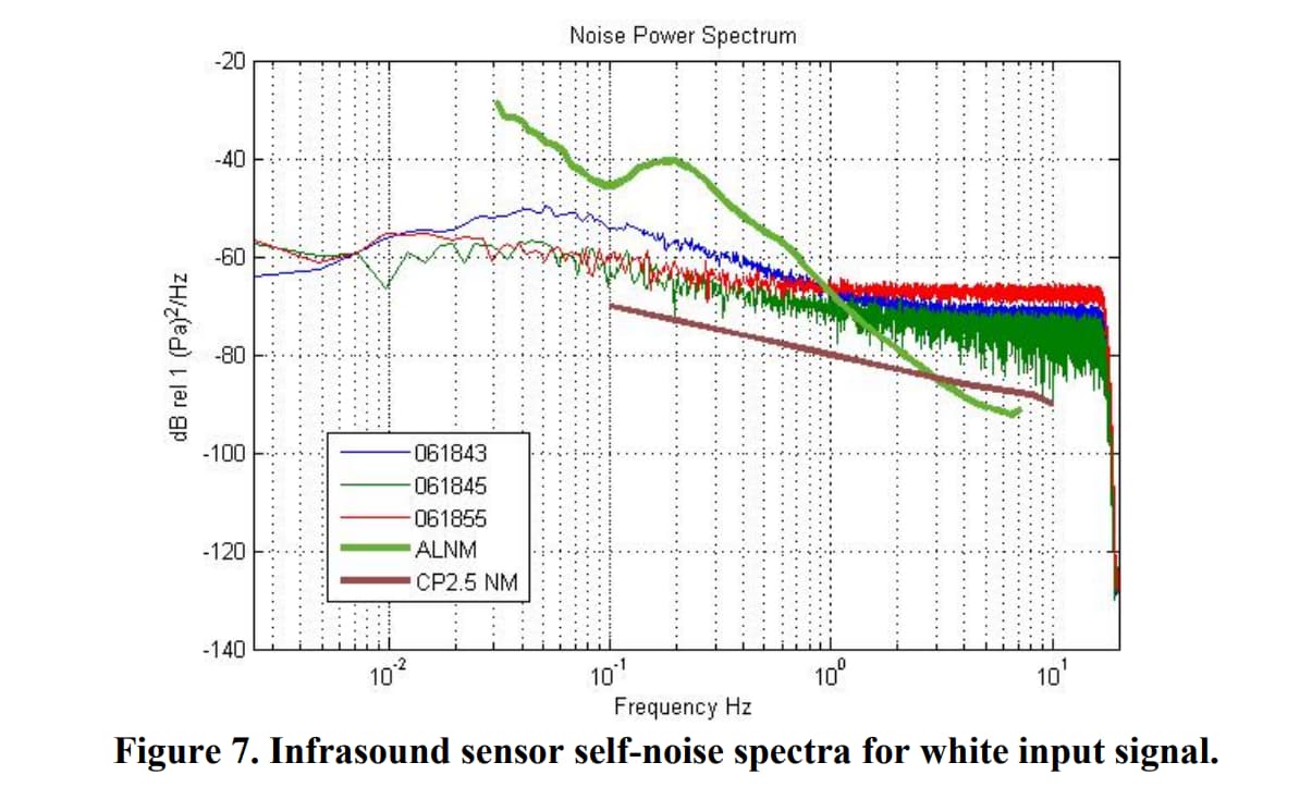
This is a power spectral density graph if I am not mistaken.

In a PSD graph the amplitude has units of power/Hz. Expressed as dB, you need to state what the zero dB reference is.
Q1: I am guessing that zero dB is 1 dB^2/Hz - can you verify?

Q2 is about the NLNM/NHNM. I could not find the origin of this for acoustic power. I did find a reference to ALNM/AHNM

07-03.PDF

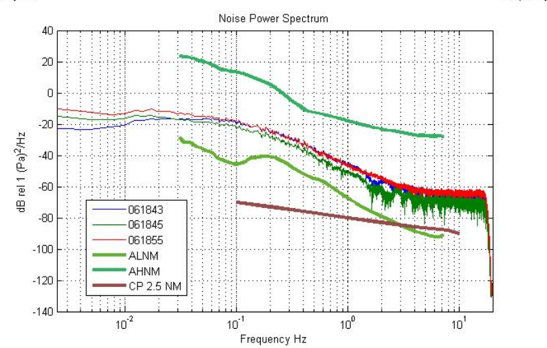
I notice in this paper, the curves for the high- and low-noise models are about 50 dB apart at 1 Hz.
In the RBoom spec they are 100 dB apart. This seems improbable. Could there be something wrong with the Y axis ?

So I guess Question 2 is about the Y-axis and the source of those curves.

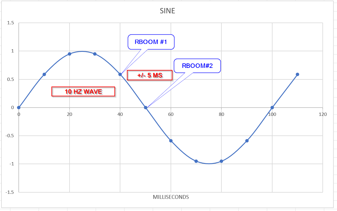
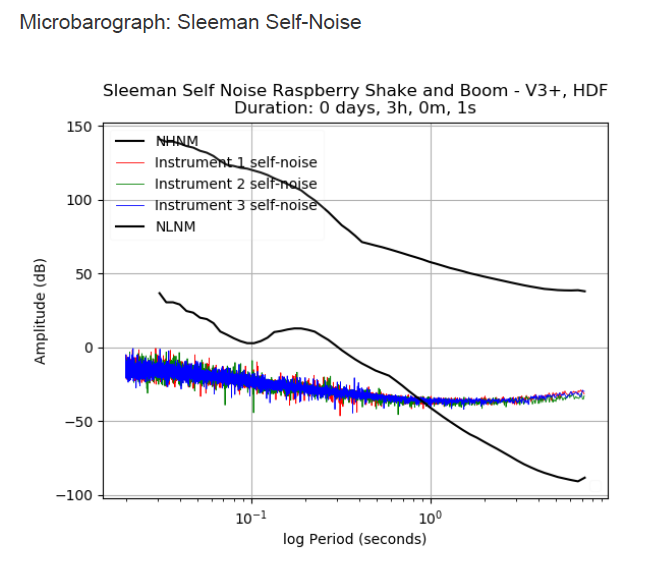
Lastly - it is noted that the RB low curve includes the digitizer. I understand the Sleeman or “three sensor correlation” technique requires the three instruments to have readings that are highly correlated. I wonder if this assumption is valid when the three RB CPU’s and A/D converters are free-running? To get fully correlated data, I would think you need to synchronize the A/D converters. Any comment?

Thanks

[branden]

@kpjamro

Q1: I have never gotten this question and do not know how to best answer you, so skipping it. Maybe @ivor knows. He has more experience with generating these models.

Q2: Source for nominal low and high infrasound noise levels:
Bowman-etal-2005-AmbientInfrasonicNoise-2005GL022486.pdf (310.3 KB)

Q3: No, there is no need to synchronize the A/D converters. Co-locating them and guaranteeing timing of +/- 1 sample (10 ms) as Raspberry Shake does is enough. That is to say, our NTP routines “synchronize” the output from the A/D converters.

branden

[kpjamro]

Thanks.

Thinking about it, the NTP sync causes the time stamps to be synchronized (if you have a local NTP server - or GPS PPS - this can be better than 1 ms. Relying on internet servers, it’s more like 10 ms as you say). Even if the A/D conversion start is aligned to the NTP PPS “instant”, you still have the time skew of NTP in your data.

Lets assume that a 10 Hertz sine wave is being recorded (at 100 SPS). What happens if the two instruments are +/- 5 milliseconds different from each other?

You can see that, when the samples retrieved for the “same” time stamp are, in fact, +/- 5 milliseconds apart, the analog values could be 50% apart at 10 Hz.

The noise calculation method depends on subtracting the analog readings, in pairs, resulting in a time series where each value is 2x the noise component and no signal component (the signal component is nulled or cancelled).

With the time resolution from NTP, you might get 3 dB nulling of signal component at 10 Hz rather than the 30 dB (or more) that is needed for a good noise estimate.

At 0.1 Hz everything is better, of course. Perhaps this is why the RB noise curve is so “flat” even curving upward at the high frequency end?

What I am saying is that the RB noise curve might be better than what you show (depending on the still unanswered questions).

[kpjamro]

Thanks. This is similar to some other papers I have found.
I also found that obspy has these curves as a built-in function somewhere.

But figure 4 and figure 6 seem to have some problems.

Figure 4 the x-axis should be 10^-1 followed by 10^0 (based on the reference to the 0.2 microbarom peak. With the axis labels on the graph it would be at 20 Hz. That’s wrong.

Figure 6 - the x-axis is as-expected but the y-axis is labeled “Pascals/Hz” whereas all the other graphs have pascals^2/Hz.

Since these are PSD’s, the y-axis should represent power - so it should be Pascals-squared.

Now, if you are still with me, looking at figure 6 you can see that, at e.g. 1 Hz, the power values span 5 orders of magnitude (approx -7 to -2) whereas the RBOOM technical spec shows 10 orders of magnitude between the high and low noise model curves.

Regards
Ken

referring to https://community.raspberryshake.org/uploads/short-url/ybBUou0miTPtX9D518Cb0Jz1nPi.pdf

edit: let me just add the observation that:

10*log(Pa^2) == 20*log(Pa)

so if you had data that was already in the format of Pa^2 and were plotting it as if it were Pa, then those numbers would be 2x what they should be (on a log scale)

That would neatly explain the situation above.

[branden]

Thanks @kpjamro

I will engage in the near future when I am back from my travels and have a moment to sit with this and think.

Very appreciative of all of your observations

branden

[kpjamro]

No rush

but another guess is the vertical axis is perhaps power and not power per Hz.

If you look at my simple self-noise test way back when:

Rboom self-noise

[self]

You see noise was 2000 counts peak-to-peak (and very flat)
2000/56000 = .0357 Pa pk-pk
assume div by 2*sqrt(2) to get RMS
.0357/2.828 = .0126 Pa RMS
20*log(.0.0126) = -38 dB (relative to 1 Pa) {20 log gives us (Pascals)^2}

If you look at https://manual.raspberryshake.org/_downloads/SpecificationsforBoom_SnB.pdf

in the vicinity of 1-10 Hz, its pretty much -38 dB. Coincidence?

The bandwidth is almost 50 Hz which is 17 dB (relative to 1 Hz)

So the normalized sensitivity is going to be around
-38-17 = -55 dB/Hz
for comparison with other devices that show PSD, rather than just noise power as a function of frequency.

Due to the instrument frequency response, the sensitivity curve will slope upwards on the left side.

cheers

[branden]

@kpjamro I really appreciate you engaging on this. I am sure we will both learn something here. And now that my vacation time with my 6 and 7 year old nieces is over, Uncle Branden has some time to engage!

Moving from the top to the bottom …

Q1: You ask what the zero dB reference is. Some background information first:

1. In seismology our “Power Spectral Density” (PSD) plots and the Nominal High and Low Noise Models represented therein come from Peterson (1993):
   https://pubs.usgs.gov/of/1993/0322/ofr93-322.pdf

2. The y-axis, more specifically, is: “Power [(10log10(m^2/sec^4/Hz)] dB”

That said, I believe that 0 dB on a seismological PSD plot corresponds to a power spectral density of 1 (um/s)^2/Hz

Q2: You ask if there could be something wrong with the Y-axis. Sure. And maybe you can check for me.

This is what I know went into generating the positioning in dB-space of the nominal reference lines in our “Microbarograph: Sleeman Self-Noise” plot:

• The original numbers were in Pa^2/Hz (see attached .txt file
  InfrasoundAmbientNoise.txt (4.2 KB)) from this paper (see attached PDF
  Bowman-etal-2005-AmbientInfrasonicNoise-2005GL022486.pdf (310.3 KB))
• This was converted by us to Period (see attached txt files:
  ISHNM.per.txt (2.1 KB)
  &
  ISLNM.per.txt (2.1 KB))

Q3: Already answered in my previous response. If you want a deeper understanding of how our NTP solution works, see: NTP and GPS timing details

branden

[kpjamro]

I am on holidays too, but will prepare more info soon.

I should first clarify that my questions pertain to the infrasound self-noise.
The Petersen paper you mention only talks about seismic noises.

There are several references online, usually related to test ban treaty monitoring.
In these references, the units of the Y axis, in the case of PSD, is Pascals^2/Hz.

Referring to the graph from the previous reference):

( [Microsoft Word - hart_50_edit_ic37au47s8s2-P (columbia.edu)]

The 0 dB refence is clearly one (pascal)^2 / Hz .
(I mistakenly said 1 dB^2/Hz above. Sorry)

I imagine other references are possible. (E.g.: 20 micropascals, the limit of human hearing)

= = = =

On NTP: this issue will be jitter. I think that in order to get the coherence you need for a Sleeman-type test arrangement, the jitter should be 2-3 orders of magnitude less than the sampling interval.

For 100 samples/sec you might need jitter < 10^-5 or 10 microseconds
The seems a stretch.

I get about 200 usec with RPI3

     remote           refid      st t when poll reach   delay   offset  jitter
====================================================================
*chronos.fios-ro .PPS.            1 u  873 1024  377    0.465   -1.308   **0.197**
 SHM(0)          .GPS.            0 l    -   16    0    0.000    0.000   0.000
 SHM(1)          .PPS.            0 l    -   16    0    0.000    0.000   0.000
+t2.time.gq1.yah 98.137.249.214   2 u  115 1024  377   67.833   -0.685   0.523
+155.248.196.28  84.168.88.243    2 u  211 1024  377   70.240    1.953   1.019
-ntp.speculation 128.9.176.30     2 u  172 1024  261   67.695    0.754   1.688

and 37 usecc with RPI4

>      remote           refid      st t when poll reach   delay   offset  jitter
> >===================================================================
> *chronos.fios-ro .PPS.            1 u  288 1024  377    0.627   -0.123   **0.037**
> +io.netbunker.or 206.108.0.131    2 u    3 1024  377   11.982    0.372   0.480
>  tick.chi1.ntfo. 206.55.64.77     3 u 134m 1024  200   21.305   -0.414   5.065
> +mx.danb.email   127.67.113.92    2 u  47m 1024  104   71.689    4.483   0.963
> ntpq>

Both are on a wired gigabit LAN.

Possibly with two RPI4’s on a gigabit LAN, the test might be valid up to 10 Hz … There is a coherence test you can do, as described in one of the USGS papers that would tell you if your testing was valid.

cheers
Ken

.

[kpjamro]

With regard to 20 micro-Pascals

There is a magic relationship (more of a convention) that 1 picowatt (10^-12 watts) of sound power will produce 20 micro-Pascals of sound pressure level over the surface of an enclosing sphere which has a surface area of 1 m^2.

I have never seen how this was derived. I think should take into account the density of air (temperature, pressure and humidity). But that seems to be ignored.

If you had a discrete machine producing some isotropic sound pressure level, and you knew the distance to the machine, you could estimate the sound power output of the machine.

In the case of a global source of sound energy, the source is quasi-infinite so calculating sound power does not work that way. And we are not trying to calculate the sound power output of Mother Nature (although I suppose someone has one that for a storm system or volcano).

What is displayed on the y-axis is a quantity that is proportional to power (watts, pressure squared, sound intensity). Normalizing it by frequency then gives a PSD graph. I have seen some Python functions that will implement this for you, if the frequency/amplitude relationship is not “flat”.

If you display two curves on the same graph, you need to ensure the reference levels are compatible and that you are using units that are proportional to power (e.g., pressure squared not pressure).

Ken