Raspberry Shake and Boom Cross Channel Correlation

sheeny · June 7, 2022, 2:58am

I’ve been playing around with different ideas to test for cross channel interference or interaction on the RS&B and finally got my head around the Cross_Correlation functions in Obspy which ATM seems by far the best way to do it compared to what I’ve tried.

This is of particular interest to me to identify and eliminate seismic sources of infrasound signal when trying to detect meteors by infrasound.

Attached is the code I’ve used FYI and use if interested. I’m sure it could be polished up and written in a more elegant manner.


from obspy.clients.fdsn import Client
from obspy.core import UTCDateTime, Stream
from obspy.signal import filter, cross_correlation
import matplotlib.pyplot as plt
rs = Client('RASPISHAKE')
xc = cross_correlation

# set the station name and download the response information
stn = 'R21C0'                            # your station name
inv = rs.get_stations(network='AM', station=stn, level='RESP')

print (inv)

# set data start/end times
start = UTCDateTime(2022, 6, 6, 23, 17, 16.7) # (YYYY, m, d, H, M, S.ffffff)
end = start + 1     # end = start + duration in seconds (S.ffffff)

# set the FDSN server location and channel names
channels = ['EHZ' , 'HDF'] # ENx = accelerometer channels; EHx or SHZ = geophone channels

# get waveforms and put them all into one Stream
stream = Stream()
for ch in channels:
        trace = rs.get_waveforms('AM', stn, '00', ch, start, end)
        stream += trace
stream.merge(method=0, fill_value='latest')
stream.detrend(type='demean')

print(stream)

#get instrument response
inv = rs.get_stations(network="AM", station=stn, level="RESP")

# setup figure and subplots
fig = plt.figure(figsize=(12,12))
ax1 = fig.add_subplot(4,1,1)
ax2 = fig.add_subplot(4,1,2)
ax3 = fig.add_subplot(4,1,3)
ax4 = fig.add_subplot(4,1,4)
fig.suptitle("AM."+stn+" RS&B Cross Channel Correlation Report: "+start.strftime('%d/%m/%Y %H:%M:%S.%f UTC'))

# plot raw traces
ax1.plot(stream[0].times(reftime=start), stream[0].data, lw=1, color='g')
ax2.plot(stream[0].times(reftime=start), stream[1].data, lw=1)

# calculate cross correlation
s = 10     # shift in data points each side to test
cc = xc.correlate(stream[0], stream[1], s)    
print(cc)         # print correlations for each shift value
shift, value = xc.xcorr_max(cc)     #find the max correlation and shift
print(shift, round(value,3))

# get the limits of the y axis so text can be consistently placed
ax2b, ax2t = ax2.get_ylim()

#add the correlation to the plot
ax2.text(0, ax2t*0.8, 'Raw Shift = '+str(shift)+'/100 s. Correlation Coefficient ='+str(round(value,3)))

# set up filter
filt = [0.3, 0.5, 10, 12]   #edit filter values to suit

# remove instrument response and add new traces to the stream
stream += stream[0].remove_response(inventory=inv,pre_filt=filt,output="VEL", water_level=60)
stream += stream[1].remove_response(inventory=inv,pre_filt=filt,output="DEF", water_level=60)

# plot filtered traces
ax3.plot(stream[0].times(reftime=start), stream[2].data, lw=1, color='r')
ax4.plot(stream[0].times(reftime=start), stream[3].data, lw=1, color='b')

#calculate cross correlation of filtered traces
cc1 = xc.correlate(stream[2], stream[3], s)    
print(cc1)         # print correlations for each shift value
shift1, value1 = xc.xcorr_max(cc1)     #find the max correlation and shift
print(shift1, round(value1,3))

# get ax4 y axis limits so text can be consistently placed
ax4b, ax4t = ax4.get_ylim()

#add the correlation to the plot
ax4.text(0, ax4t*0.8, 'Filtered Shift = '+str(shift1)+'/100 s. Correlation Coefficient ='+str(round(value1,3)))

# setup some plot details
ax1.set_ylabel("EHZ Raw Counts")
ax2.set_ylabel("HDF Raw Counts")         
ax3.set_ylabel("EHZ Velocity (m/s) ("+str(filt[1])+" to "+str(filt[2])+"Hz)")
ax4.set_ylabel("HDF Pascals (Pa) ("+str(filt[1])+" to "+str(filt[2])+"Hz)")

# save the final figure
#plt.savefig(stn+' RSandB Corr'+start.strftime('%Y%m%d %H%M%S UTC'))  #comment this line out till figure is final

# show the final figure
plt.show()

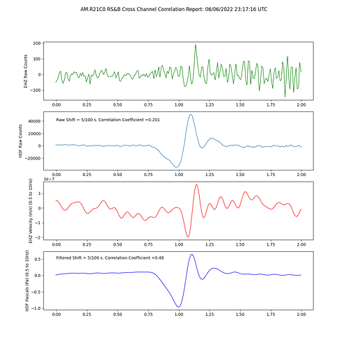
This is what the output looks like:

In this case, there’s a 48% correlation between the filtered EHZ and HDF channels and as the HDF signal is leading the EHZ channel by 0.05s it appears to be the HDF channel influencing the EHZ channel.

This obviously works best for short sections of signal. Long sections are likely to reduce the correlation as random noise becomes more significant.

Al.

Stormchaser · June 7, 2022, 8:47am

Another very interesting product sheeny, thank you for sharing it with us in the community!

I look forward to testing it as soon as I can move my SB in a less noisier location.

sheeny · June 7, 2022, 9:26am

I have just replaced the code with a slight update to facilitate durations of less than 1 second, so the start time can be specified with decimal seconds and the duration can be a short as required.

I’ve had some interesting results testing it so far. I picked some obvious events that are common to both EHZ and HDF channels and was surprised couple of times to find the correlation reduced with a 0.5 to 10 Hz bandpass rather than increased. This of course just means the interaction is in frequencies outside that range. For meteors the frequency range I’m interested in is 0.5 to 10 Hz so it was a pleasant surprise to see an obvious correlation that was essentially in what would be considered noise (when looking for meteors).

Al.

sheeny · June 8, 2022, 2:21am

I have just replaced the code again with another minor update to consistently position the shift and correlation text in the plot figures.

Its worth noting that this application still requires a bit of interpretation from the user. The Obspy Cross Correlation function is designed for comparing similar seismic data on different stations. In this application we are using it to compare seismic with infrasound, so the biggest differences are in signal scale due to different units and counts and speed of transmission of signals.

I’ll share here my thoughts on interpretation that I’ve built my experimentation so far.

There are 4 scenarios that lead to an apparent correlation or interaction of seismic and infrasound signal in the RS&B:

seismic signals that are strong enough to generate an infrasound signal or otherwise affect the infrasound detector;
infrasound signals that are strong enough to affect the geophone;
local events which generate both seismic and infrasound signals;
external interference (RF, magnetic, or electrical) which may affect the Raspberry Pi or the sensors or other components of the RS&B.

So far, from what I’ve found, a strong seismic signal should produce the best correlation with a negative shift and likewise a strong infrasound signal should produce a the best correlation with a positive shift. A positive shift means the infrasound signal leads, and vice versa. Zero shift, obviously suggests simultaneous signals.

Type 3 events should produce best correlation with a negative shift (seismic excitation of the infrasound (if any) arrives before genuine infrasound signal but any infrasound signal doesn’t necessarily have to match the seismic signal. For example, I tested signals for several passing log trucks. The road is approx 100m from the RS&B. Despite, the HDF and EHZ signals both obviously being from the truck, the correlation was relatively to very low. So even though the signals are related to the same event, the signals are largely independent. Local impacts or explosions (events that are likely to produce a similar shaped signal in both ground and air waves) might be very different to this.

So far I haven’t detected any events that I could attribute to RF, magnetic or electrical interference. This may be the most likely source of zero shift correlations depending on what part of the system the interference is affecting.

I would also suggest that if a shift is encountered equal to the maximum value of s, that the value of s be increased to broaden the possible range of shifts the correlation function is calculated over. i.e. the best correlation may be outside the range set by +/- s.

Al.