Hello,
I am trying to get power spectral density (PSD) data from specific time frames of ambient data on my Raspberry Shake 3D (v7). I have extracted the sensitivity, poles, and zeros from the SeisComp version of the response file here. I have been playing with the obspy ppsd module and matplotlib psd and specgram modules.
The Obspy PPSD appears to work somewhat. Looking at the technical docs (specifically, pg. 13-16), it seems like I should be able to get reasonable data from (for example) 0.5-10 Hz (0.1-2 s period).
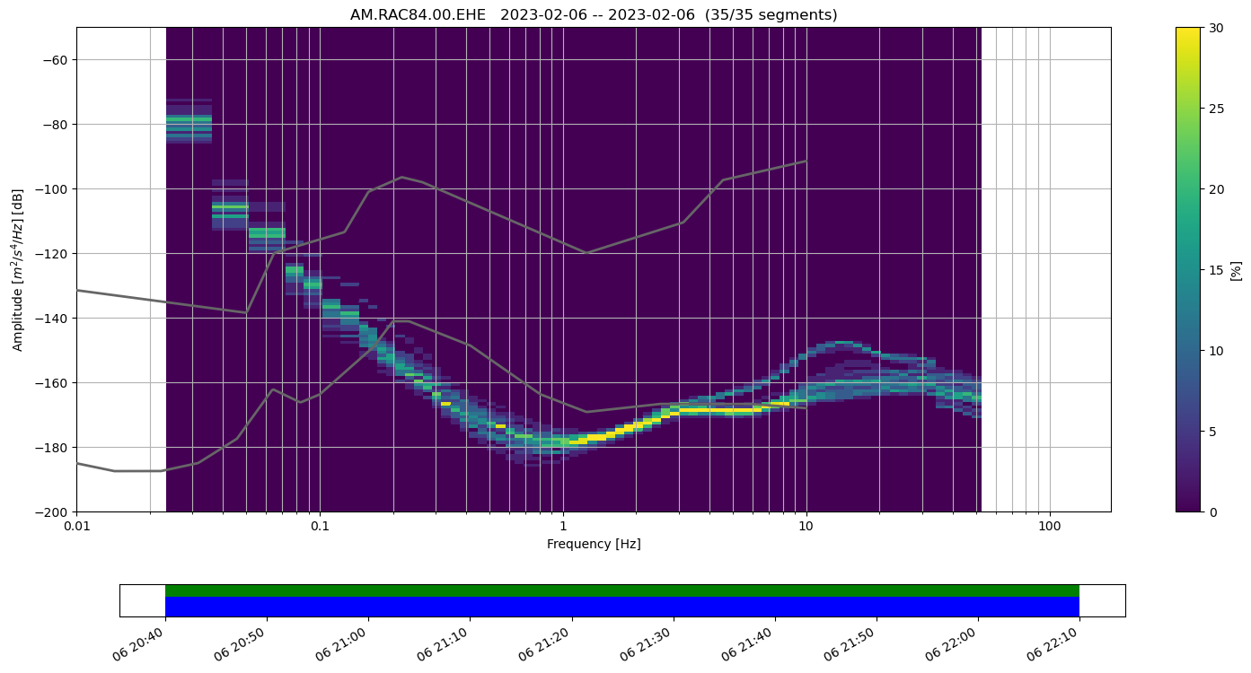
I collected some test data recently for a couple of hours (my shake is in offline mode, using GPS for timing) and ran obspy.ppsd following the example they show on their website, I seem to get reasonable ppsd values between 0.3 - 9+ Hz. Around 0.3ish Hz and lower the ppsd values appear to deteriorate in terms of their usefulness/reasonableness, and none of the lower frequency data appears to be useful. According to the NHNM and NLNM data, this is also rather small in terms of the amplitude axis.
(See code and images below)
The plots also look a little funny to me when running the matplotlib modules too, though with some slightly different issues.
When I use the psd, there appears to also be a change in the character of the data below 0.4 Hz (or maybe as high as 2 Hz?).(See code and images below)
When I use the specgram module, there appears to be a change in the data around perhaps 2 Hz? Or maybe even more so at 0.4 Hz. (See code and images below)
Basically, the question I have is whether this is an instrument limitation, or if I need to figure out a better way to install/place the Shake (or process the data!). I do not claim to be a master seismologist (I’m still learning), but I think all the processing/plotting inputs, etc. make sense?
It may be worth noting, I had a commercial seismometer sitting next to this one during this same time period, and I was able to process across the entire spectra mentioned above. I won’t upload the data because it is a proprietary format, but it has helped me see what I ‘should’ be getting out, and it seems to work fine.
The paz response information I am using are below, all read from the response file mentioned above.
paz= {
‘sensitivity’:360000000.0,
‘gain’:360000000.0,
‘poles’: [(-1+0j),
(-1+0j),
(-3.03+0j),
(-3.03+0j),
(-3.03+0j),
(-3.03+0j),
(-666.67+0j),
(-666.67+0j)],
‘zeros’: [0j, 0j, 0j, 0j, 0j, 0j]
}
The data I am using is here:
AM.RAC84.00.EH_.D.2023.zip (2.6 MB)
Some code snippets, in case that is helpful:
import datetime
import pathlib
import time
import obspy
from obspy.signal import PPSD
import numpy as np
invFile = filepath_to_response_file

#I have a function here to update the response file with the correct station name, etc.
inv = obspy.read_inventory(invFile, format='STATIONXML', level='response')
paz = function_to_extract_paz #See actual paz variable above

filepaths = [filepathZ, filepathN, filepathE]

traceList = []
for i, f in enumerate(filepaths):
    st = obspy.read(str(f))
    tr = (st[0])
    traceList.append(tr)
inStream = obspy.Stream(traceList)
inStream.attach_response(inv)

trimStart = obspy.UTCDateTime(datetime.datetime(2023,02,06,20,40))
trimEnd = obspy.UTCDateTime(datetime.datetime(2023,02,06,22,10))

stream = inStream.copy()
stream.trim(starttime=trimStart, endtime=trimEnd)

ppsd = PPSD(stream[0].stats, paz, ppsd_length=300, overlap=0.5)
ppsd.add(stream)
ppsd.plot(xaxis_frequency=True) #This gives the  output below
Output:
Now, the matplotlib modules:
import matplotlib.pyplot as plt
trz = obspy.read(path_to_zTrace)
trn = obspy.read(path_to_nTrace)
tre = obspy.read(path_to_eTrace
#Bandpass filter
bpFilt = [0.01, 0.02, 15, 20]
invFile = filepath_to_response_file
#I have a function here to update the response file with the correct station name, etc.
inv = obspy.read_inventory(invFile, format='STATIONXML', level='response')
trz = trz[0].remove_response(inventory=inv, pre_filt=bpFilt)
trn = trn[0].remove_response(inventory=inv, pre_filt=bpFilt)
tre = tre[0].remove_response(inventory=inv, pre_filt=bpFilt)
traceList = [trz, trn, tre]
st = obspy.Stream(traceList)
#You could do this for each trace, they're all similar
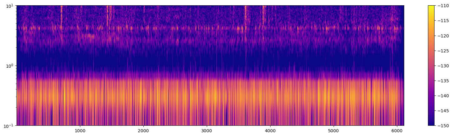
spectrumz, freqsz, tz, imz = plt.specgram(trz, Fs=100, detrend='mean', scale='dB', NFFT=512,
vmin=-150, vmax=-110, cmap='plasma')
plt.ylim([0.1,10])
plt.semilogy()
plt.colorbar()
Output:
This is what I would expect very generally from about 0.8 Hz or so and higher, but below 0.8 Hz, it seems odd (it might even be odd starting around 2 Hz, it’s hard to tell? Again, I’m no expert, trying to learn).
And now for the psd:
import matplotlib as plt
trz = obspy.read(path_to_zTrace)
trn = obspy.read(path_to_nTrace)
tre = obspy.read(path_to_eTrace

#Bandpass filter
bpFilt = [0.01, 0.02, 15, 20]

invFile = filepath_to_response_file

#I have a function here to update the response file with the correct station name, etc.

inv = obspy.read_inventory(invFile, format='STATIONXML', level='response')

trz = trz[0].remove_response(inventory=inv, pre_filt=bpFilt)
trn = trn[0].remove_response(inventory=inv, pre_filt=bpFilt)
tre = tre[0].remove_response(inventory=inv, pre_filt=bpFilt)

pxxz, freqsz = plt.psd(trz, detrend='linear', Fs=100, NFFT=6000, return_line=False, label='Z',
                                             noverlap=30)
pxxn, freqsn = plt.psd(trn, detrend='linear', Fs=100, NFFT=6000, return_line=False, label='N',
                                             noverlap=30)
pxxe, freqse = plt.psd(tre, detrend='linear', Fs=100, NFFT=6000, return_line=False, label='E',
                                             noverlap=3000)

plt.legend()
plt.semilogx()
plt.ylim([-175, -75])
plt.xlim([0.1, 10])
Output:
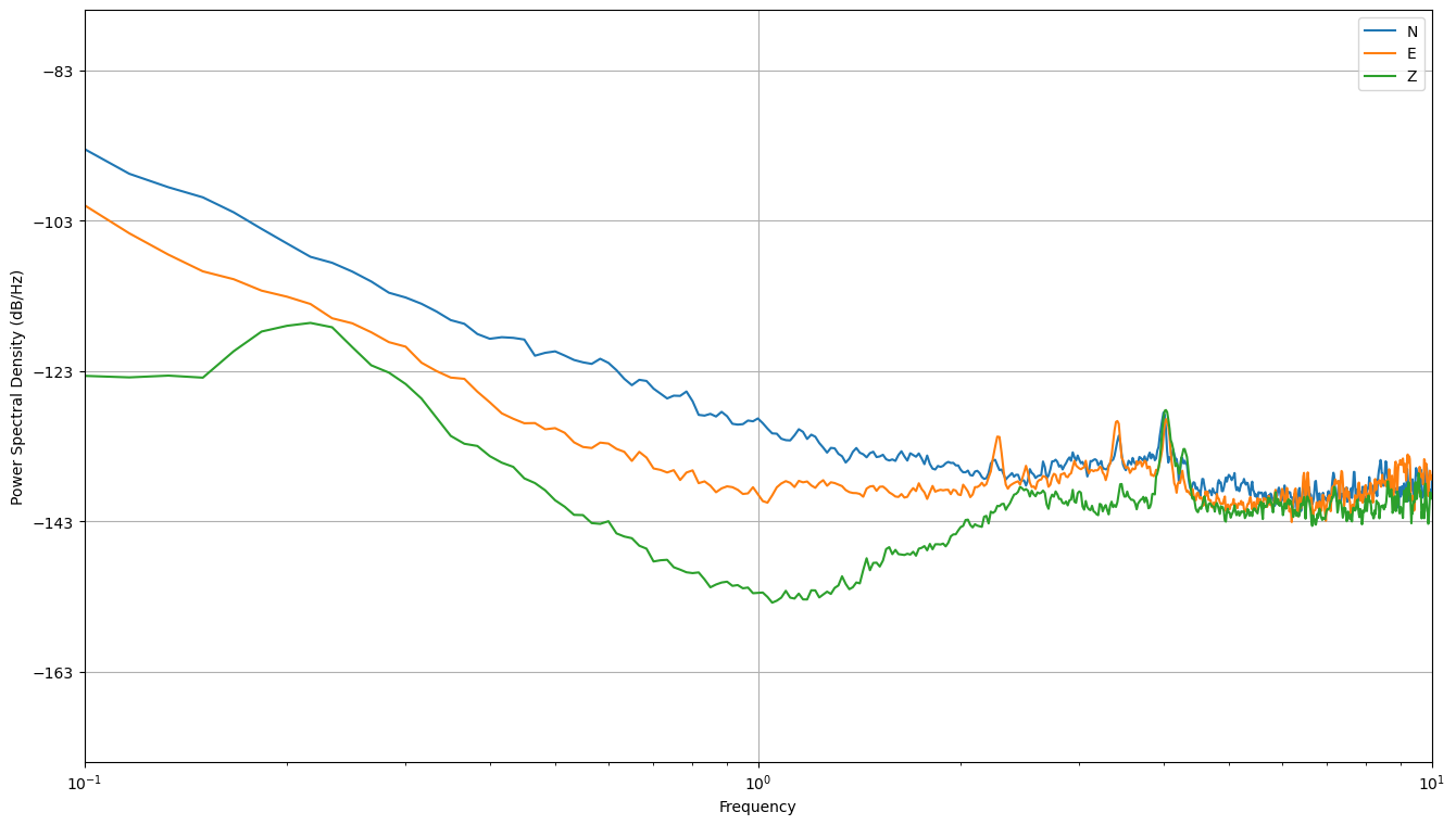
This is maybe what I expect down to maybe 0.4 Hz (may be actually more around 2 Hz), then everything lower than that I’m not sure about.