Plotting travel time on a Section Plot

I’m trying to plot arrival time curves onto a section plot, and not having any success. I know other’s have done it, but I’ve exhausted all my ideas for now.

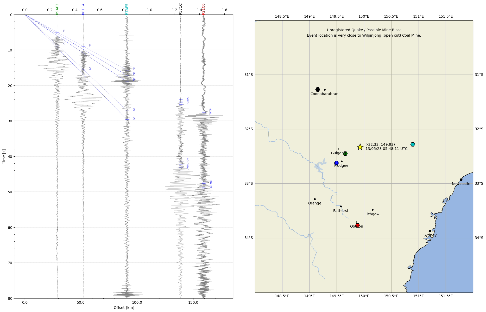
My idea was to make a crude program for finding small local quakes that aren’t on ShakeNet or other sources. I’ve observed a few interesting events like this now. The idea is to adjust the time and location of the quake until the arrival time curves match the waveform plots.

Here’s what the report looks like ATM with the plot_travel_times line commented out.

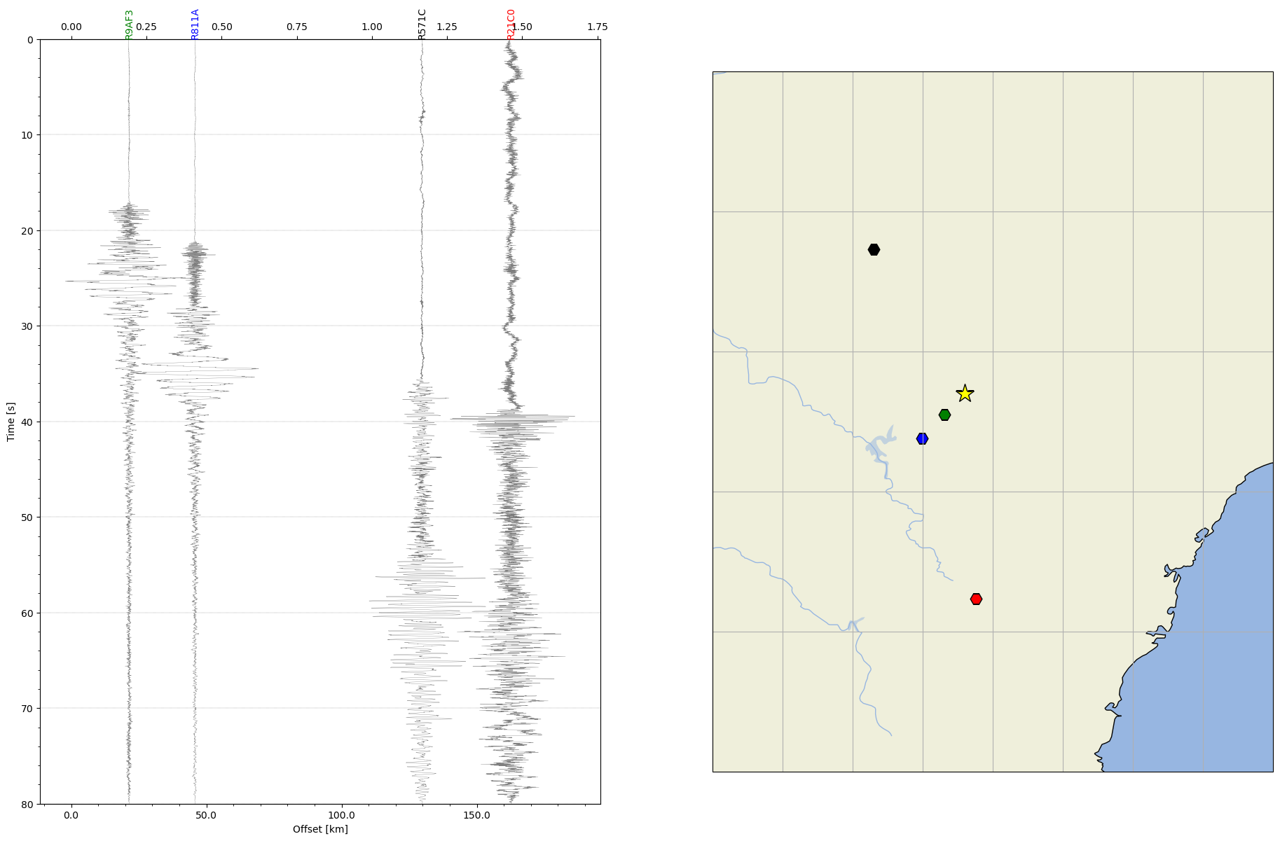
I’m struggling to get the plot_travel_times line to work.

This is my code:


# -*- coding: utf-8 -*-
"""
Created on Sun May 21 12:22:53 2023

@author: al72
"""

from obspy.clients.fdsn import Client
from obspy.core import UTCDateTime, Stream
#from obspy.signal import filter
import matplotlib.pyplot as plt
#from matplotlib.ticker import AutoMinorLocator
#import numpy as np
from obspy.taup import TauPyModel, plot_travel_times
#import math
import cartopy.crs as ccrs
import cartopy.feature as cfeature
from matplotlib.transforms import blended_transform_factory
from obspy.geodetics import gps2dist_azimuth, kilometers2degrees, degrees2kilometers

rs = Client('https://data.raspberryshake.org/')

def stationList(sl):
    sl += ['R21C0']
    sl += ['R811A']
    sl += ['R9AF3']
    sl += ['R571C']
    #sl += ['R6D2A']
    #sl += ['RF35D']
    #sl += ['R7AF5']
    #sl += ['R3756']
    #sl += ['R6707']
    #sl += ['RB18D']
    #print(sl)
    return sl
    
def freqFilter(ft):
    # bandpass filter - select to suit system noise and range of quake
    #ft = [0.1, 0.1, 0.8, 0.9]
    #ft = [0.3, 0.3, 0.8, 0.9]
    #ft = [0.5, 0.5, 2, 2.1]
    ft = [0.7, 0.7, 2, 2.1]       #distant quake
    #ft = [0.7, 0.7, 3, 3.1]
    #ft = [0.7, 0.7, 4, 4.1]
    #ft = [0.7, 0.7, 6, 6.1]
    #ft = [0.7, 0.7, 8, 8.1]
    #ft = [1, 1, 10, 10.1]
    #ft = [1, 1, 20, 20.1]
    #ft = [3, 3, 20, 20.1]        #use for local quakes
    #print(ft)
    return ft
 
def buildStream(strm):
    n = len(slist)
    print(n)
    for i in range(0, n):
        inv = rs.get_stations(network='AM', station=slist[i], level='RESP')  # get the instrument response
        #print(inv[0])
        
        #read each epoch to find the one that's active for the event
        k=0
        while True:
            sta = inv[0][k]         #station metadata
            if sta.is_active(time=eventTime):
                break
            k += 1
        latS = sta.latitude     #active station latitude
        lonS = sta.longitude     #active station longitude
        #eleS = sta.elevation     #active station elevation
        #print(slist[i], latS, lonS)
        #print(sta)
        trace = rs.get_waveforms('AM', station=slist[i], location = "00", channel = 'EHZ', starttime = start, endtime = end)
        trace.merge(method=0, fill_value='latest')         #fill in any gaps in the data to prevent a crash
        trace.detrend(type='demean')                       #detrend the data
        tr1 = trace.remove_response(inventory=inv,zero_mean=True,pre_filt=filt,output='VEL',water_level=.001, plot=False) # convert to Vel
        tr1[0].stats.distance = gps2dist_azimuth(latS, lonS, latE, lonE)[0]
        tr1[0].stats.latitude = latS
        tr1[0].stats.longitude = lonS
        tr1[0].stats.colour = colours[i]
        strm += tr1
    #strm.plot(method='full', equal_scale=False)
    return strm

def k2d(x):
    return kilometers2degrees(x)

def d2k(x):
    return degrees2kilometers(x)
    
eventTime = UTCDateTime(2023, 5, 13, 5, 48, 00) # (YYYY, m, d, H, M, S) **** Enter data****
latE = -32.3                           # quake latitude + N -S **** Enter data****
lonE = 149.8                        # quake longitude + E - W **** Enter data****
depth = 1                             # quake depth, km **** Enter data****
mag = 1                              # quake magnitude **** Enter data****
eventID = 'unknown'               # ID for the event **** Enter data****
locE = "Mudgeeish, NSW, Australia"                # location name **** Enter data****

slist = []
filt = []
stationList(slist)
freqFilter(filt)
colours = ['r', 'b', 'g', 'k', 'c', 'm', 'purple', 'orange', 'gold', 'midnightblue']
#print(slist)
#print(filt)

#set up the plot
delay = 0
duration = 80
start = eventTime + delay
end = start + duration

st = Stream()
buildStream(st)
#print(st)

#set up the figure
fig = plt.figure(figsize=(20,14), dpi=100)       # set to page size in inches

#build the section plot
ax1 = fig.add_subplot(1,2,1)
st.plot(type='section', plot_dx=50e3, recordlength=80, time_down=True, linewidth=.25, grid_linewidth=.25, show=False, fig=fig)
# Plot customization: Add station labels to offset axis
ax = ax1.axes
transform = blended_transform_factory(ax.transData, ax.transAxes)
for t in st:
    ax.text(t.stats.distance / 1e3, 1.0, t.stats.station, rotation=90,
            va="bottom", ha="center", color=t.stats.colour, transform=transform, zorder=10)

#setup secondary x axis
secax_x1 = ax1.secondary_xaxis('top', functions = (k2d, d2k))

#plot arrivals times
model = TauPyModel(model="iasp91")
#ax = plot_travel_times(source_depth=1, ax=ax, fig=fig, max_degrees=1.6, phase_list=['P', 'S'])

#plot the map
ax2 = fig.add_subplot(1,2,2, projection=ccrs.PlateCarree())
ax2.set_extent([148,152,-35,-30], crs=ccrs.PlateCarree())
#ax2.coastlines(resolution='110m')
#ax2.stock_img()
# Create a features
states_provinces = cfeature.NaturalEarthFeature(
    category='cultural',
    name='admin_1_states_provinces_lines',
    scale='50m',
    facecolor='none')
ax2.add_feature(cfeature.LAND)
ax2.add_feature(cfeature.OCEAN)
ax2.add_feature(cfeature.COASTLINE)
ax2.add_feature(states_provinces, edgecolor='gray')
ax2.add_feature(cfeature.LAKES, alpha=0.5)
ax2.add_feature(cfeature.RIVERS)
ax2.gridlines()
#plot event/earthquake position on map
ax2.plot(lonE, latE,
     color='yellow', marker='*', markersize=20, markeredgecolor='black',
     transform=ccrs.Geodetic(),
     )
#plot station positions on map
for tr in st:
    ax2.plot(tr.stats.longitude, tr.stats.latitude,
             color=tr.stats.colour, marker='H', markersize=12, markeredgecolor='black',
             transform=ccrs.Geodetic(),
             )
    ax2.plot

plt.show()

Line 134 is the problem. I’ve tried every permutation I can think of, so hoping some else has done this and can point me in the right direction.

Thanks,

Al.

1 Like

Hello Al,

I have not used that function, so I cannot be 100% sure, but I think that the issue is that you are trying to plot, on the same figure, two charts with different axes:

  1. Your waveform chart that has x[axis] = Offset [km] and y[axis] = Time [s]
  2. The arrival times that has x[axis] = Distance [degrees] and y[axis] = Time [min]

To see this, you can temporarily substitute line 134 with this:

ax = plot_travel_times(source_depth=1, max_degrees=1.6, phase_list=['P', 'S'], fig=fig)

and see both charts plotted one above the other in a strange mashup.

You will have to either 1) adjust the axes of the first chart so that they match the second, or 2) vice-versa so that, with all axes matching, you can then plot them together on the same figure.

Otherwise, Python doesn’t know how to do the conversion between the two and generates mashups or the straight-up errors that you have seen.

Maybe you can take inspiration from Mark Vanstone’s code here: GitHub - wmvanstone/RPiShakeCode: Python code for accessing seismic data from Raspberry Shake and BGS networks that has lots of sample section plots.

1 Like

G’Day Stormchaser.

Thanks for the link to Mark Vanstone’s code. There’s a lot of good examples there.

I’ve done some playing about trying to transform the plots to match without success. I have had an idea for another way to go about it which should avoid the whole transformation problem, and a see that that is what Mark has done in some of his programs. It just goes to show that sometimes the “obvious” way to do something is not the easiest.

Thanks for your help!

Al.

2 Likes

Always welcome Al!

Looking forward to your results.

Here’s the preliminary result:

This unregistered quake is very close to an Open Cut coal mine. The coordinates in the model ATM are that of one of the pits in the mine. The fit is trial and error both in time and position (and depth).

I found that at some depths Obspy does not produce any arrivals less than some figure below 0.8 of a degree, so I added some straight line plots from the origin to 0.8° for those cases.

Here’s the code so far if anyone is interested:


# -*- coding: utf-8 -*-
"""
Created on Sun May 21 12:22:53 2023

@author: al72
"""

from obspy.clients.fdsn import Client
from obspy.core import UTCDateTime, Stream
#from obspy.signal import filter
import matplotlib.pyplot as plt
#from matplotlib.ticker import AutoMinorLocator
#import numpy as np
from obspy.taup import TauPyModel
#import math
import cartopy.crs as ccrs
import cartopy.feature as cfeature
from matplotlib.transforms import blended_transform_factory
from obspy.geodetics import gps2dist_azimuth, kilometers2degrees, degrees2kilometers

rs = Client('https://data.raspberryshake.org/')

def stationList(sl):
    sl += ['R21C0']
    sl += ['R811A']
    sl += ['R9AF3']
    sl += ['R571C']
    #sl += ['R6D2A']
    #sl += ['RF35D']
    sl += ['R7AF5']
    #sl += ['R3756']
    #sl += ['R6707']
    #sl += ['RB18D']
    #print(sl)
    return sl
    
def freqFilter(ft):
    # bandpass filter - select to suit system noise and range of quake
    #ft = [0.1, 0.1, 0.8, 0.9]
    #ft = [0.3, 0.3, 0.8, 0.9]
    #ft = [0.5, 0.5, 2, 2.1]
    ft = [0.7, 0.7, 2, 2.1]       #distant quake
    #ft = [0.7, 0.7, 3, 3.1]
    #ft = [0.7, 0.7, 4, 4.1]
    #ft = [0.7, 0.7, 6, 6.1]
    #ft = [0.7, 0.7, 8, 8.1]
    #ft = [1, 1, 10, 10.1]
    #ft = [1, 1, 20, 20.1]
    #ft = [3, 3, 20, 20.1]        #use for local quakes
    #print(ft)
    return ft
 
def buildStream(strm):
    n = len(slist)
    #print(n)
    for i in range(0, n):
        inv = rs.get_stations(network='AM', station=slist[i], level='RESP')  # get the instrument response
        #print(inv[0])
        
        #read each epoch to find the one that's active for the event
        k=0
        while True:
            sta = inv[0][k]         #station metadata
            if sta.is_active(time=eventTime):
                break
            k += 1
        latS = sta.latitude     #active station latitude
        lonS = sta.longitude     #active station longitude
        #eleS = sta.elevation     #active station elevation
        #print(slist[i], latS, lonS)
        #print(sta)
        trace = rs.get_waveforms('AM', station=slist[i], location = "00", channel = 'EHZ', starttime = start, endtime = end)
        trace.merge(method=0, fill_value='latest')         #fill in any gaps in the data to prevent a crash
        trace.detrend(type='demean')                       #detrend the data
        tr1 = trace.remove_response(inventory=inv,zero_mean=True,pre_filt=filt,output='VEL',water_level=.001, plot=False) # convert to Vel
        tr1[0].stats.distance = gps2dist_azimuth(latS, lonS, latE, lonE)[0]
        tr1[0].stats.latitude = latS
        tr1[0].stats.longitude = lonS
        tr1[0].stats.colour = colours[i]
        strm += tr1
    #strm.plot(method='full', equal_scale=False)
    return strm

def k2d(x):
    return kilometers2degrees(x)

def d2k(x):
    return degrees2kilometers(x)

places = [['Oberon', -33.704922, 149.862900, 2],
          ['Bathurst', -33.419281, 149.577499, 4],
          ['Lithgow', -33.480930, 150.157410, 4],
          ['Mudgee', -32.590439, 149.588684, 4],
          ['Orange', -33.283333, 149.100006, 4],
          ['Sydney', -33.868820, 151.209290, 6],
          ['Newcastle', -32.926670, 151.780014, 6],
          ['Coonabarabran', -31.273911, 149.277420, 4],
          ['Gulgong', -32.362492, 149.532104, 2]
          ]
    
eventTime = UTCDateTime(2023, 5, 13, 5, 48, 11) # (YYYY, m, d, H, M, S) **** Enter data****
latE = -32.33                           # quake latitude + N -S **** Enter data****
lonE = 149.93                        # quake longitude + E - W **** Enter data****
depth = 0                             # quake depth, km **** Enter data****
mag = 1                              # quake magnitude **** Enter data****
eventID = 'unknown'               # ID for the event **** Enter data****
locE = "Mudgeeish, NSW, Australia"                # location name **** Enter data****

slist = []
filt = []
stationList(slist)
freqFilter(filt)
colours = ['r', 'b', 'g', 'k', 'c', 'm', 'purple', 'orange', 'gold', 'midnightblue']
plist = ('P', 'S')
#print(slist)
#print(filt)

#set up the plot
delay = 0
duration = 80
start = eventTime + delay
end = start + duration

st = Stream()
buildStream(st)
#print(st)

#set up the figure
fig = plt.figure(figsize=(20,14), dpi=100)       # set to page size in inches

#build the section plot
ax1 = fig.add_subplot(1,2,1)
st.plot(type='section', plot_dx=50e3, recordlength=80, time_down=True, linewidth=.25, grid_linewidth=.25, show=False, fig=fig)

# Plot customization: Add station labels to offset axis
ax = ax1.axes
transform = blended_transform_factory(ax.transData, ax.transAxes)
for t in st:
    ax.text(t.stats.distance / 1e3, 1.0, t.stats.station, rotation=90,
            va="bottom", ha="center", color=t.stats.colour, transform=transform, zorder=10)

#setup secondary x axis
secax_x1 = ax1.secondary_xaxis('top', functions = (k2d, d2k))

#plot arrivals times
model = TauPyModel(model="iasp91")
#ax = plot_travel_times(source_depth=1, ax=ax, fig=fig, max_degrees=1.6, phase_list=['P', 'S'])

for t in st:
    arr = model.get_travel_times(depth, k2d(t.stats.distance/1000), phase_list=plist)
    n = len(arr)
    #print(arr)
    for i in range(0,n):
        ax.plot(t.stats.distance/1000, arr[i].time, marker='_', markersize=10, color = 'b', alpha=0.5)
        ax.text(t.stats.distance/1000+5, arr[i].time, arr[i].name, color='b', alpha=0.5)
       
arr = model.get_travel_times(depth, 0.8, phase_list=plist)
n = len(arr)
for i in range(0,n):
    ax.plot([0,d2k(0.8)], [0, arr[i].time], linestyle = '--', linewidth=0.5, color='b', alpha=0.5)

#plot the map
ax2 = fig.add_subplot(1,2,2, projection=ccrs.PlateCarree())
ax2.set_extent([148,152,-35,-30], crs=ccrs.PlateCarree())
#ax2.coastlines(resolution='110m')
#ax2.stock_img()
# Create a features
states_provinces = cfeature.NaturalEarthFeature(
    category='cultural',
    name='admin_1_states_provinces_lines',
    scale='50m',
    facecolor='none')
ax2.add_feature(cfeature.LAND)
ax2.add_feature(cfeature.OCEAN)
ax2.add_feature(cfeature.COASTLINE)
ax2.add_feature(states_provinces, edgecolor='gray')
ax2.add_feature(cfeature.LAKES, alpha=0.5)
ax2.add_feature(cfeature.RIVERS)
ax2.gridlines(draw_labels=True)
#plot event/earthquake position on map
ax2.plot(lonE, latE,
     color='yellow', marker='*', markersize=20, markeredgecolor='black',
     transform=ccrs.Geodetic(),
     )
ax2.text(lonE+0.1, latE-0.05, "("+str(latE)+", "+str(lonE)+")\n"+eventTime.strftime('%d/%m/%y %H:%M:%S UTC'))

#plot station positions on map
for tr in st:
    ax2.plot(tr.stats.longitude, tr.stats.latitude,
             color=tr.stats.colour, marker='H', markersize=12, markeredgecolor='black',
             transform=ccrs.Geodetic(),
             )

#plot places
for pl in places:
    ax2.plot(pl[2], pl[1], color='k', marker='o', markersize=pl[3], markeredgecolor='k', transform=ccrs.Geodetic(), label=pl[0])
    ax2.text(pl[2], pl[1]-0.1, pl[0], horizontalalignment='center', transform=ccrs.Geodetic())

#add notes to map
ax2.text(150, -30.2, 'Unregistered Quake / Possible Mine Blast', ha='center')
ax2.text(150, -30.3, 'Event location is very close to Wilpinjong (open cut) Coal Mine.', ha='center')

plt.subplots_adjust(wspace=0.1)

plt.show()

It’s by no means final. I’ll tinker with it to pretty it up and make it more adaptable to other applications. I have another unregistered quake that only showed up on 3 local shakes last year to tackle as well.

Al.

2 Likes

I was just seeing this on Twitter, and I have to say that it’s a great preliminary result Al!

The P & S waves for the closest Shakes are very prominent and clear, and I think that this is an overall solid foundation to continue building on, as you have said.

Thanks also for sharing the code with the community!

The P&S waves aren’t too bad on the later two as well but the one in the middle, R7AF5, not so much. I wonder if that’s a function of the direction of the bench and the sequence of the blast (if it was a blast)?

Al.

2 Likes