If you have freshly re-installed Anaconda you shouldn’t need this check, but please verify that you are using the latest version (23.3.1). From the command line, you can use conda -V or conda --version to get your current conda version.
After this, you don’t need to import any package in the PPV environment. The command
will automatically create a new environment named ppvmotion and download/install all required packages/modules. I’ve just tested it on my Anaconda installation on Win11 and everything appears to work fine.
Starting over - it works. Although, I did not figure out where the .ipynb files were.
Instead I just copy/pasted the text of the github file, and filled in the needed spots, and it works on an R3D.
I changed it so that it only asks for one channel - EHZ - and I can make a plot for my system.
Actually, there are three rows in the plot, with just the top graph filled in.
If I set nrows = 1, it throws an error at me. I don’t know how to make only one graph.
But that is pretty good progress for the first day.
I think the way that Obspy should work is that it looks at the instrument XML file finds if the instrument reads in M or M/S or M/S^2 and then integrates or differentiates as needed so that all three outputs can be produced (ACC, VEL or DISP).
yes?
In that case, PPV should simply use the VEL output. The trick with PPV is that, strictly speaking, you need three dimensions and do the Pythagorean sum to find which point in time has the greatest velocity along some diagonal. With an RS1, you only have one axis so it is simple.
The other requirement I have seen is that you say what frequency is associated with the peak. In one reference they suggest finding the waveform zero crossing on either side of the peak and measuring the time between zeros. The inverse of that is the approximate frequency. I don’t know how to do that in Obspy.
BTW - I found why the ACC graph was so low - the sample code had the bandpass filter applied after the conversion to ACC. You need to filter the instrument output before doing the differentiation.
All right kpjamro, lots of progress here, great work!
Let’s proceed step-by-step:
Copy-pasting is more than enough in the end, so it was good thinking on your part.
If you want to plot a single channel (EHZ, in your case) you will have to adapt the code a bit. Just replace the block from line 38 to line 67 with the following:
    # generate figure
    fig, ax = plt.subplots(figsize=(20, 10), nrows=1, ncols=1)
    fig.tight_layout(pad=3.0)

    # plot peak particle velocity charts for each channel of the RS3D unit
    if len(list(sta)) == 3:
        # download and process waveforms for each channel
        st = client.get_waveforms(network, station, loc, val, starttime=start_time, endtime=end_time, attach_response=True)
        st.merge(method=0, fill_value='latest')
        st.detrend(type="demean")
        st.filter("bandpass", freqmin=f1, freqmax=f2, corners=cor)
        st.remove_response(output="DISP")

        # beautify the plots
        ax.plot(st[0].times(reftime=start_time), 2*np.pi*freq*st[0].data*1000, lw=1)
        ax.margins(x=0.0001)
        ax.grid(color='dimgray', ls = '-.', lw = 0.33)
        ax.set_ylabel("Peak Particle Velocity (mm/s)")
        ax.set_xlabel("Time after Start (s)")
        staleg = str(station + " - " + val + " - " + "Filter: bandpass " + str(f1) + " - " + str(f2) + " Hz")
        ax.legend([staleg])

        # save the final figure
        plt.savefig("PPVMotion_" + station + ".png")
    else:

        # if unit is not a RS3D, warn the user
        print("Please insert a RS3D Station.")
The instrument output is always in raw Counts, a unitless number that is essentially an analogue for the amount of voltage on the circuit of the given channel at the given time. (IRIS: Frequently Answered Question ). ObsPy then reads both this data and the instrument response file to output appropriate converted Counts to m (DISP), m/s (VEL), or m/s**2 (ACC).
With the formula that is used in this code from the cited source (https://www.castlegroup.co.uk/ground-vibration/), the a parameter is in mm; thus DISP is required. If, however, you will be using a different formula, feel free to adapt the conversion to suit your needs.
With regard to point 4 the formula: the cited source imagines that your wave is sinusoidal and that you know the frequency of it. With 100 sps the maximum the wave frequency could be is just under 50 Hz. But, in the example, it is filtered down to a maximum of 2 Hz (and may be as low as 0.7). If you plug in 100 Hz for the frequency, you overestimate the velocity by a factor of at least 50 times (100/2) . I won’t comment more on that other than to suggest using “f2” instead of “freq” as a more realistic value for that approach.
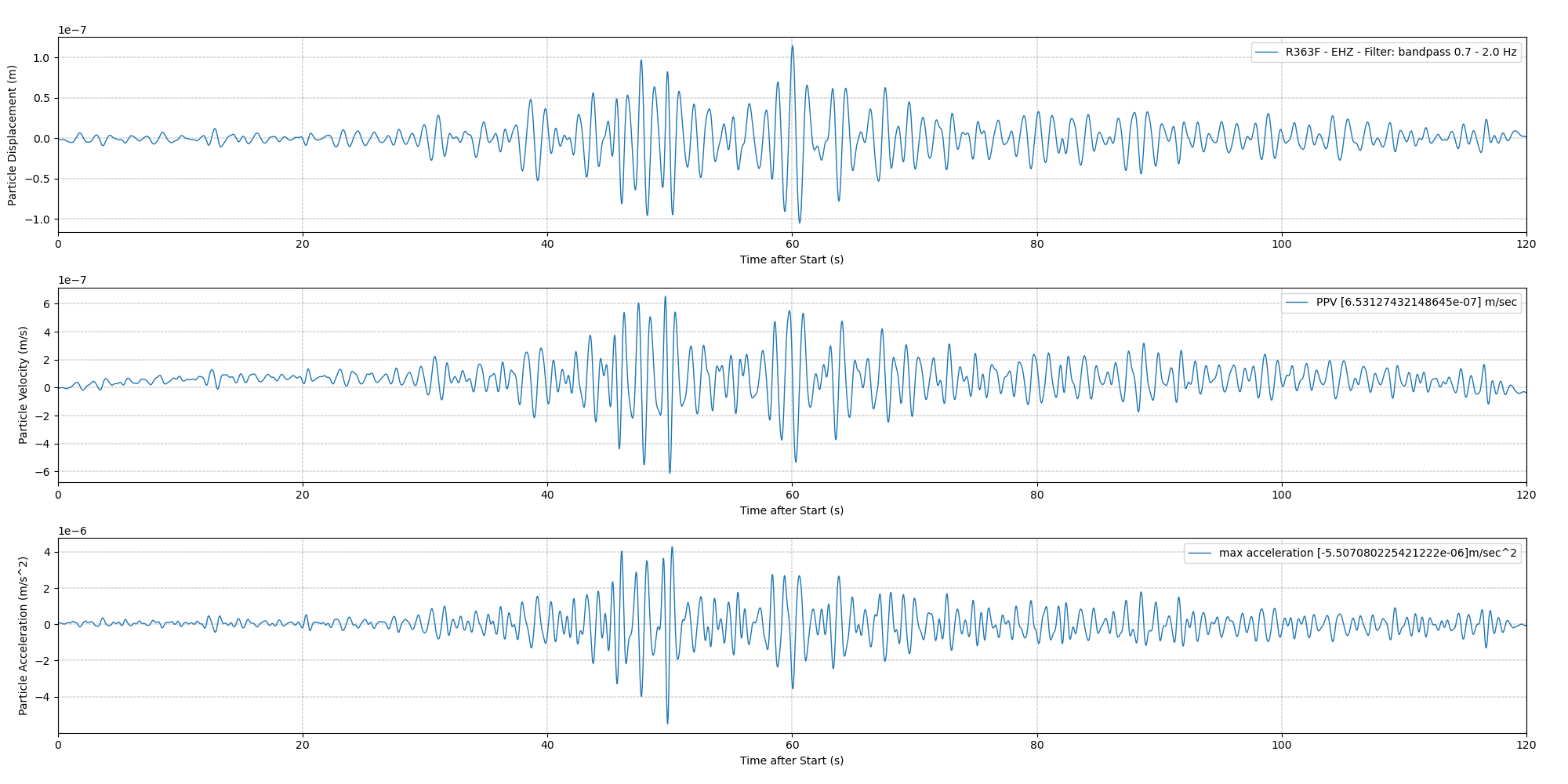
In my case, it seemed best just to ask Ospby to give me the velocity directly and use the trace max function to find the maximum value. I produced three graphs - one for displacement, one for velocity (with max - which is the PPV) and one for acceleration (with max):
I would like fewer decimal digits but this will do for now.
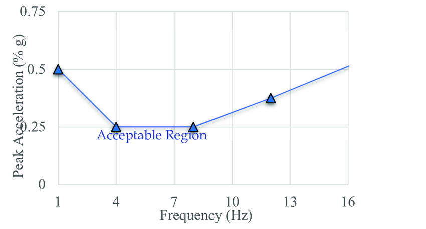
I will also scale velocity to be in inches/second which is what local codes require and to express acceleration in fractional percent of gravity - since that seems often used when describing human sensitivity to vibration.
Regarding the decimal values, you can round the variable you want to display (PPV, max acceleration, etc.) with this:
round(PPV,2)
where PPV is your variable, and the number after the comma is the number of decimal values you want to display. You can adjust this to suit your needs.
Regarding the rest, this is great work! As it could be of interest to other users too, when you finish optimizing your code, could you post it here in full? So that there will be a good reference point for other interested parties in the future.
it is possible that the previous mymax value was interpreted as a list for some reason. I cannot be more precise without seeing the code that generates it.
The second part seems to do what you had in mind. I imagine that the PPV values will always be small numbers, so they should match what you need?
The code seemed wrong to me and misleading. @kpjamro above has already indicated why.
PPV is simply the peak of the VEL ouput. Simply plot VEL to see the peak (PPV). That’s it.
However, the repo code takes the DISP and integrates it to obtain the VEL. The integration seems wrong, because although it correctly uses the 2 pi freq formula, it is using the 100 Hz for the frequency due to the 100 sps rather than the frequency of the waveform.
Also, kpjamro says that “strictly speaking, you need three dimensions and do the Pythagorean sum” but actually British Standards used for construction-related vibration (BS 7385, BS 5228, etc) take PPV to be the largest velocity in any of the measured orthogonal directions.
It would be nice if someone could correct if I’ve made an errors in this post. Maybe I’ll submit some code as a new post once progressed.
These are very interesting observations. Thank you for taking the time to elaborate on what you’ve seen.
As this is one of our public repos, feel free to update the code yourself with the version you deem most suitable compared to the current one. We are always looking at anything that can improve what we offer.