Local "quakes" and estimating Magnitude

[sheeny]

I thought I’d share my latest incarnation of code for small local quakes. I’ve been playing with this for a while but have finally developed the code for estimating the magnitude (ML) for small local quakes using the Tsuboi Estimation Formula.

I use this code for both known local quakes and to locate small quakes that aren’t registered on other systems that appear of 3 or more local stations.

The code contains a lot of data that is unique to me and my local stations, but this can be replaced with the equivalent data for any location as required. For example, latitudes and longitudes for any town world wide can be found at https://www.latlong.net/

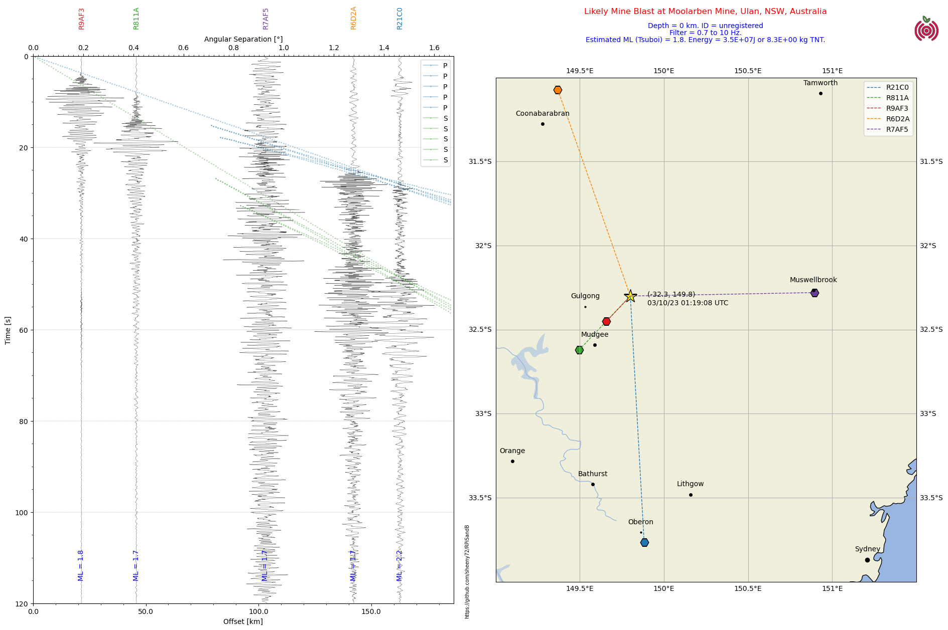
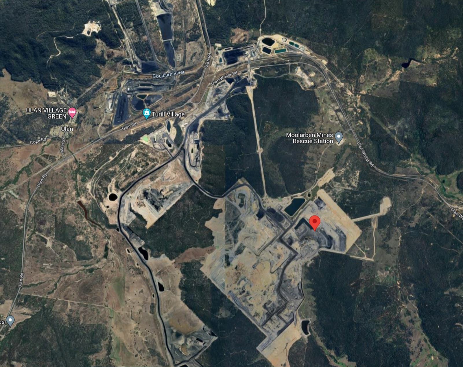
Here’s an example for a mine blast that I found on my shake this morning, and then found the corresponding signal on neighbouring shakes as well. Trial and error soon locates the time and place of the quake - in this case it coincides with the Moolarben Coal Mine near Ulan.

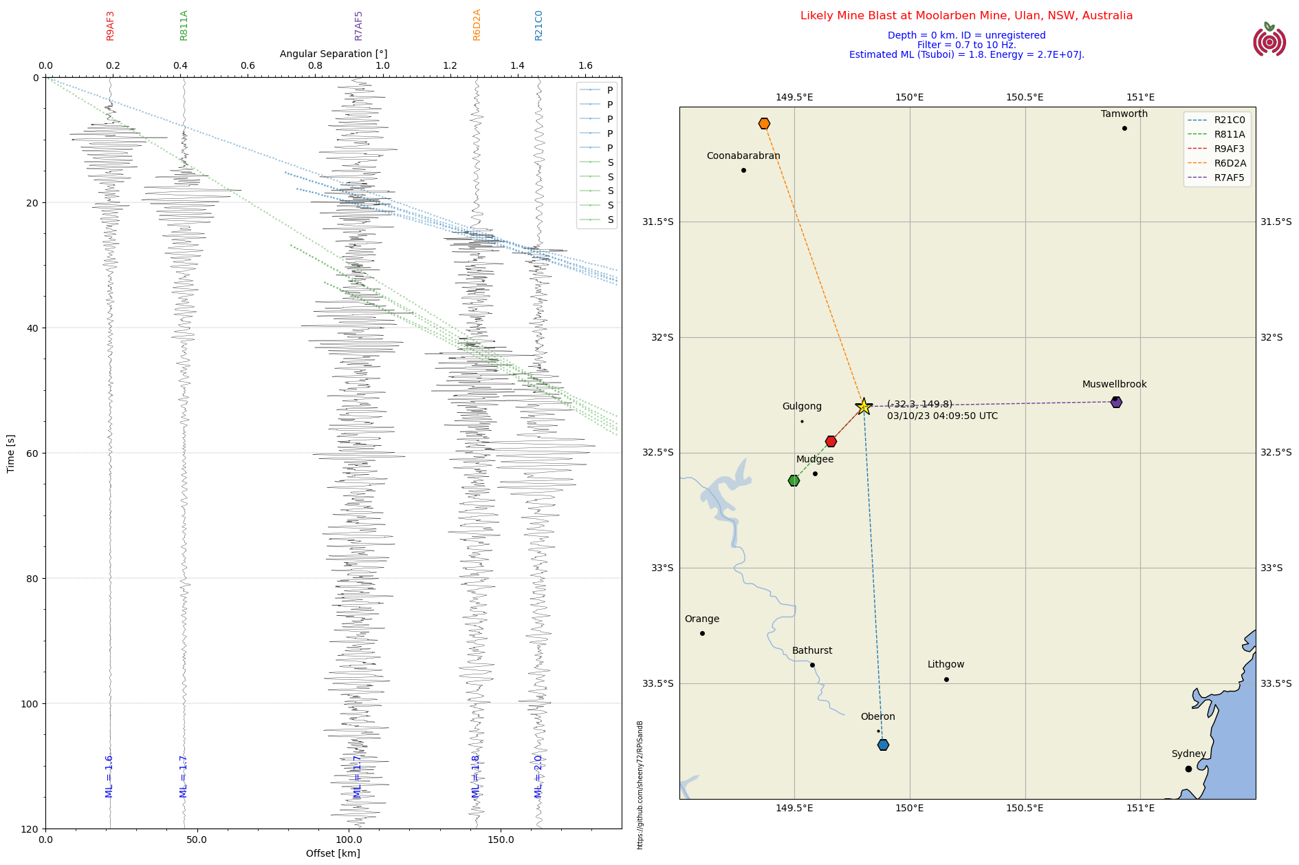
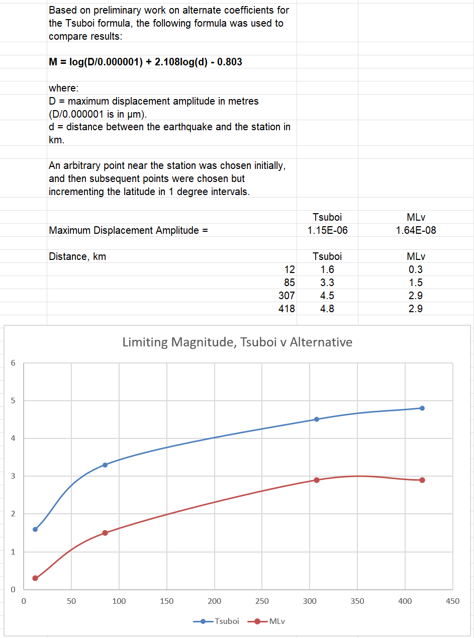
I chose the Tsuboi estimation formula for it’s simplicity. It just requires the maximum displacement amplitude of the signal and the distance to the epicentre to calculate. By changing my section plot from velocity traces to displacement traces the maximum displacement amplitude is easily found, and the epicentral distance is calculated anyway for the section plot.

Here’s the code:

# -*- coding: utf-8 -*-
"""
Created on Sun May 21 12:22:53 2023

@author: al72
"""

from obspy.clients.fdsn import Client
from obspy.core import UTCDateTime, Stream
import matplotlib.pyplot as plt
from obspy.taup import TauPyModel
import cartopy.crs as ccrs
import cartopy.feature as cfeature
import numpy as np
from matplotlib.transforms import blended_transform_factory
from matplotlib.cm import get_cmap
from obspy.geodetics import gps2dist_azimuth, kilometers2degrees, degrees2kilometers
from matplotlib.ticker import AutoMinorLocator

rs = Client('https://data.raspberryshake.org/')

# Build a station list of local stations so unwanted stations can be commented out
# as required to save typing
def stationList(sl):
    sl += ['R21C0']     #Oberon
    sl += ['R811A']     #Mudgee
    sl += ['R9AF3']    #Gulgong
    #sl += ['R571C']     #Coonabarabran
    sl += ['R6D2A']    #Coonabarabran
    #sl += ['RF35D']    #Narrabri
    sl += ['R7AF5']     #Muswellbrook
    #sl += ['R26B1']     #Murrumbateman
    #sl += ['R3756']    #Chatswood
    #sl += ['R9475']    #Sydney
    #sl += ['R6707']    #Gungahlin
    #sl += ['R69A2']    #Penrith
    #sl += ['RB18D']     #Canberra
    #sl += ['R9A9D']    #Brisbane
    #sl += ['RCF6A']    #Brisbane
    #sl += ['S6197']     #Heyfield
    #sl += ['RD371']    #Melbourne
    #sl += ['RC98F']    #Creswick
    #sl += ['RA20F']    #Broken Hill
    #sl += ['RC74C']    #Broken Hill
    #print(sl)
    return sl

# Build a stream of traces from each of the selected stations    
def buildStream(strm):
    n = len(slist)      # n is the number of traces (stations) in the stream
    tr1 = []
    for i in range(0, n):
        inv = rs.get_stations(network='AM', station=slist[i], level='RESP')  # get the instrument response
        
        #read each epoch to find the one that's active for the event
        k=0
        while True:
            sta = inv[0][k]         #station metadata
            if sta.is_active(time=eventTime):
                break
            k += 1
        latS = sta.latitude     #active station latitude
        lonS = sta.longitude     #active station longitude
        #eleS = sta.elevation     #active station elevation is not required for this program
        print(sta)      # print the station on the console so you know which, if any, station fails to have data
        trace = rs.get_waveforms('AM', station=slist[i], location = "00", channel = '*HZ', starttime = start, endtime = end) #vertical geophone could be EHZ or SHZ
        trace.merge(method=0, fill_value='latest')         #fill in any gaps in the data to prevent a crash
        trace.detrend(type='demean')                       #detrend the data
        tr1 = trace.remove_response(inventory=inv,zero_mean=True,pre_filt=ft,output='DISP',water_level=60, plot=False) # convert to displacement so ML can be estimated
        # save data in the trace.stats for use later
        tr1[0].stats.distance = gps2dist_azimuth(latS, lonS, latE, lonE)[0] # distance from the event to the station in metres
        tr1[0].stats.latitude = latS        # save the station latitude from the inventory with the trace
        tr1[0].stats.longitude = lonS       # save the station longitude from the inventory with the trace
        tr1[0].stats.colour = colours[i % len(colours)]    # assign a colour to the station/trace
        tr1[0].stats.amp = np.abs(tr1[0].max()/1e-6)   # max displacement amplitude in µm
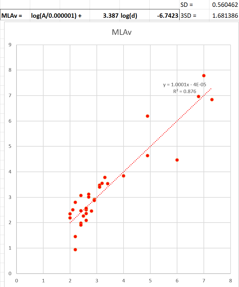
        tr1[0].stats.mL = np.log10(tr1[0].stats.amp) + 1.73*np.log10(tr1[0].stats.distance/1000) - 0.83   #ML by Tsuboi Empirical Formula
        strm += tr1
    #strm.plot(method='full', equal_scale=False)
    return strm

# function to convert kilometres to degrees
def k2d(x):
    return kilometers2degrees(x)

# function to convert degrees to kilometres
def d2k(x):
    return degrees2kilometers(x)

# Build a list of local places for the map
# Lat Long Data from https://www.latlong.net/
# format ['Name', latitude, longitude, markersize]
#comment out those not used to minimise typing
places = [['Oberon', -33.704922, 149.862900, 2],
          ['Bathurst', -33.419281, 149.577499, 4],
          ['Lithgow', -33.480930, 150.157410, 4],
          ['Mudgee', -32.590439, 149.588684, 4],
          ['Orange', -33.283333, 149.100006, 4],
          ['Sydney', -33.868820, 151.209290, 6],
          #['Newcastle', -32.926670, 151.780014, 5],
          #['Wollongong', -34.427811, 150.893066, 5],
          ['Coonabarabran', -31.273911, 149.277420, 4],
          ['Gulgong', -32.362492, 149.532104, 2],
          #['Narrabri', -30.325060, 149.782974, 4],
          ['Muswellbrook', -32.265221, 150.888184, 4],
          ['Tamworth', -31.092749, 150.932037, 4],
          #['Boorowa', -34.437340, 148.717972, 2],
          #['Cowra', -33.828144, 148.677856, 4],
          #['Dubbo', -32.246380, 148.591263, 4],
          #['Goulburn', -34.754539, 149.717819, 4],
          #['Cooma', -36.235291, 149.125275, 4],
          #['Grafton', -29.690960, 152.932968, 4],
          #['Coffs Harbour', -30.296350, 153.115692, 4],
          #['Armidale', -30.512960, 151.669418, 4],
          #['Brisbane', -27.469770, 153.025131, 6],
          #['Canberra', -35.280937, 149.130005, 6],
          #['Albury', -36.073730, 146.913544, 4],
          #['Wagga Wagga', -35.114750, 147.369614, 4],
          #['Broken Hill', -31.955891, 141.465347, 4],
          #['Wilcannia', -31.558981, 143.378464, 4],
          #['Cobar', -31.494930, 145.840164, 4],
          #['Melbourne', -37.813629, 144.963058, 6]
          ]

# Enter event data (estimate by trial and error for unregistered events)    
eventTime = UTCDateTime(2023, 10, 3, 4, 9, 50) # (YYYY, m, d, H, M, S) **** Enter data****
latE = -32.3                                    # quake latitude + N -S **** Enter data****
lonE = 149.8                                    # quake longitude + E - W **** Enter data****
depth = 0                             # quake depth, km **** Enter data****
mag = 0                              # quake magnitude **** Enter data****
eventID = 'unregistered'               # ID for the event **** Enter data****
locE = "Moolarben Mine, Ulan, NSW, Australia"      # location name **** Enter data****

slist = []
stationList(slist)
# bandpass filter - select to suit system noise and range of quake
#ft = [0.09, 0.1, 0.8, 0.9]
#ft = [0.29, 0.3, 0.8, 0.9]
#ft = [0.49, 0.5, 2, 2.1]
#ft = [0.6, 0.7, 2, 2.1]       #distant quake
#ft = [0.6, 0.7, 3, 3.1]
#ft = [0.6, 0.7, 4, 4.1]
#ft = [0.6, 0.7, 6, 6.1]
#ft = [0.6, 0.7, 8, 8.1]
#ft = [0.9, 1, 10, 10.1]
ft = [0.69, 0.7, 10, 10.1]
#ft = [0.9, 1, 20, 20.1]
#ft = [2.9, 3, 20, 20.1]        #use for local quakes
# Pretty paired colors. Reorder to have saturated colors first and remove
# some colors at the end. This cmap is compatible with obspy taup - credit to Mark Vanstone for this code.
cmap = get_cmap('Paired', lut=12)
colours = ['#%02x%02x%02x' % tuple(int(col * 255) for col in cmap(i)[:3]) for i in range(12)]
colours = colours[1:][::2][:-1] + colours[::2][:-1]
print(colours)
#colours = ['r', 'b', 'g', 'k', 'c', 'm', 'purple', 'orange', 'gold', 'midnightblue']    # array of colours for stations and phases
plist = ('P', 'S')      # phase list for plotting

#set up the plot
delay = 0           # for future development for longer distance quakes - leave as 0 for now!
duration = 120       #adjust duration to get detail required
start = eventTime + delay   # for future development for longer distance quakes
end = start + duration      # for future development for longer distance quakes

# Build the stream of traces/stations
st = Stream()
buildStream(st)

#set up the figure
fig = plt.figure(figsize=(20,14), dpi=100)       # set to page size in inches

#build the section plot
ax1 = fig.add_subplot(1,2,1)
st.plot(type='section', plot_dx=50e3, recordlength=duration, time_down=True, linewidth=.3, alpha=0.8, grid_linewidth=.25, show=False, fig=fig)

# Plot customization: Add station labels to offset axis
ax = ax1.axes
transform = blended_transform_factory(ax.transData, ax.transAxes)
axt, axb = ax1.get_ylim()   #get the top and bottom limits of the axes
#print(axt, axb)
j=0
mLav = 0
for t in st:
    ax.text(t.stats.distance / 1e3, 1.05, t.stats.station, rotation=90,
            va="bottom", ha="center", color=t.stats.colour, transform=transform, zorder=10)
    ax.text(t.stats.distance / 1e3, axt-5, 'ML = '+str(np.round(t.stats.mL,1)), rotation=90,
            va="bottom", ha="center", color = 'b', zorder=10)    #print ML estimates
    mLav += t.stats.mL  
    j += 1

#calculate average ML estimate
mLav = mLav/j

#Calculate Earthquake Total Energy
qenergy = 10**(1.5*mLav+4.8)

#setup secondary x axis
secax_x1 = ax1.secondary_xaxis('top', functions = (k2d, d2k))   #secondary axis in degrees separation
secax_x1.set_xlabel('Angular Separation [°]')
secax_x1.xaxis.set_minor_locator(AutoMinorLocator(10))

#plot arrivals times
model = TauPyModel(model="iasp91")

axl, axr = ax1.get_xlim()   # get the left and right limits of the section plot
if axl<0:           #if axl is negative, make it zero to start the range for phase plots
    axl=0
#axl = 300      # uncomment to adjust left side of section plot, kms
ax1.set_xlim(left = axl)
for j in range (int(axl), int(axr)):    # plot phase arrivals every kilometre
    arr = model.get_travel_times(depth, k2d(j), phase_list=plist)
    n = len(arr)
    for i in range(0,n):
        if j == int(axr)-1:
            ax.plot(j, arr[i].time, marker='o', markersize=1, color = colours[plist.index(arr[i].name) % len(colours)], alpha=0.3, label = arr[i].name)
        else:
            ax.plot(j, arr[i].time, marker='o', markersize=1, color = colours[plist.index(arr[i].name) % len(colours)], alpha=0.3)
#        if j/50 == int(j/50):       # periodically plot the phase name
#            ax.text(j, arr[i].time, arr[i].name, color=colours[plist.index(arr[i].name) % len(colours)], alpha=0.5, ha='center', va='center')
    j+=1
ax.legend(loc = 'best')
                
#plot the map
ax2 = fig.add_subplot(1,2,2, projection=ccrs.PlateCarree())
mt = -31    # latitude of top of map
mb = -34    # latitude of the bottom of the map
ml = 149    # longitude of the left side of the map
mr = 151.5    # longitude of the right side of the map
ax2.set_extent([ml,mr,mt,mb], crs=ccrs.PlateCarree())
#ax2.coastlines(resolution='110m')  # use for large scale maps
#ax2.stock_img()                    # use for large scale maps

# Create a features
states_provinces = cfeature.NaturalEarthFeature(
    category='cultural',
    name='admin_1_states_provinces_lines',
    scale='50m',
    facecolor='none')
ax2.add_feature(cfeature.LAND)
ax2.add_feature(cfeature.OCEAN)
ax2.add_feature(cfeature.COASTLINE)
ax2.add_feature(states_provinces, edgecolor='gray')
ax2.add_feature(cfeature.LAKES, alpha=0.5)
ax2.add_feature(cfeature.RIVERS)
ax2.gridlines(draw_labels=True)
#plot event/earthquake position on map
ax2.plot(lonE, latE,
     color='yellow', marker='*', markersize=20, markeredgecolor='black',
     transform=ccrs.Geodetic(),
     )
# print the lat, long, and event time beside the event marker
ax2.text(lonE+0.1, latE-0.05, "("+str(latE)+", "+str(lonE)+")\n"+eventTime.strftime('%d/%m/%y %H:%M:%S UTC'))

#plot station positions on map
for tr in st:
    ax2.plot(tr.stats.longitude, tr.stats.latitude,
             color=tr.stats.colour, marker='H', markersize=12, markeredgecolor='black',
             transform=ccrs.Geodetic(),
             )
    ax2.plot([tr.stats.longitude, lonE], [tr.stats.latitude, latE],
         color=tr.stats.colour, linewidth=1, linestyle='--', 
         transform=ccrs.Geodetic(), label = tr.stats.station,
         )
ax2.legend()

#plot places
for pl in places:
    ax2.plot(pl[2], pl[1], color='k', marker='o', markersize=pl[3], markeredgecolor='k', transform=ccrs.Geodetic(), label=pl[0])
    ax2.text(pl[2], pl[1]+0.05, pl[0], horizontalalignment='center', transform=ccrs.Geodetic())

#add Notes
#fig.text(0.75, 0.96, 'M'+str(mag)+' Earthquake at '+locE, ha='center', size = 'large', color='r')  # use for identified earthquakes
fig.text(0.75, 0.96, 'Likely Mine Blast at '+locE, ha='center', size = 'large', color='r')     # use for unidentified events
fig.text(0.75, 0.94, 'Depth = '+str(depth)+' km. ID = '+eventID, ha='center', color = 'b')
fig.text(0.75, 0.93, 'Filter = '+str(ft[1])+' to '+str(ft[2])+' Hz.', ha='center', color = 'b')
fig.text(0.75, 0.92, 'Estimated ML (Tsuboi) = '+str(np.round(mLav,1))+'. Energy = '+f"{qenergy:0.1E}"+'J.', ha='center', color = 'b')

# add github repository address for code
fig.text(0.51, 0.1,'https://github.com/sheeny72/RPiSandB', size='x-small', rotation=90)

# plot logos
rsl = plt.imread("RS logo.png")
newaxr = fig.add_axes([0.935, 0.915, 0.05, 0.05], anchor='NE', zorder=-1)
newaxr.imshow(rsl)
newaxr.axis('off')

plt.subplots_adjust(wspace=0.1)

# add a plt.savefig(filename) line here if required.

plt.show()

I have made other code examples of mine available for use on Github: sheeny72 (Alan Sheehan) · GitHub

Enjoy,

Al.

[Stormchaser]

This is an amazing work Al, fantastic!!

Thank you for sharing your code with all the community too! I am curious to see (when I have the time to do something with it) how it performs with the shakes on the W coast of Scotland and the very small quakes that happen there.

Again, thank you!

[sheeny]

Thanks Stormchaser, no worries.

Like a lot of things in seismology it’s not precise. I suspect these sort of methods probably work best with unfiltered spectrograms and the algorithm caters for the attenuation of higher frequencies with distance.

If you look at the example above you can see there’s a general trend of increasing magnitude with distance. I think that’s because I’ve applied it to filtered (0.7 to 10Hz) spectrograms, so I’m losing some amplitude off the signal close to the event. Just something to keep in mind. It’s a trade off - under estimate by using filtered spectrograms or possibly over estimate by including noise in unfiltered spectrograms. Maybe its best to use the biggest result rather than the average? I don’t know. Maybe with time we’ll get a feel for it. I’ll have to try it on some quakes with known magnitude and see.

Either way its better than nothing to give some sort of idea of the size of the event when that’s not available elsewhere.

Al.

[sheeny]

Here’s the results of a quick experiment with filters.

In this case the upper filter limit did not change the magnitude estimate if I increased it from 10 (i.e. I tried 10, 20, 40 and 50 Hz). I did not expect that. I thought that might explain the trend in values in this example, but it doesn’t.

I then experimented with the lower filter limit from 0.3 up to 0.7 and that has an effect on the magnitude but the average is pretty consistent for “good looking” spectrograms i.e. not dominated by low frequency swings. 0.5Hz was a reasonable lower limit (in this case), below that the magnitude increased and the spectrograms looked pretty ugly.

So the Tsuboi Estimation Formula is more robust that I expected.

Al.

[sheeny]

Found another likely blast a few hours before the first one I posted:

I’ve also written this Tsuboi Estimation Formula into my normal quake report, so we’ll see how it compares to the official magnitudes. So far on a the few examples I’ve tried it seems to underestimate the magnitude - at least on larger magnitudes that I’ve tried.

Al.

[sheeny]

A thought occurred to me this morning about why the Tsuboi formula might be estimating the magnitude low. I’m applying it to the vertical EHZ channel, but the horizontal channels typically have greater amplitude than vertical.

It may be more accurate on the horizontal channels of a 3D or 4D shake.

Al.

[ivor]

hi,

just to be complete, the channel which will have the greater amplitude depends on the angle of arrival, where more oblique will see greater amplitudes on the horizontals, while more acute (er, less oblique) will see greater amplitudes on the vertical.

since the hypocenter of most EQs will not be located close to directly below the receiver (seismometer), it is true to say that the horizontal channels will typically contain the larger recordings of ground motion (a more oblique angle of approach), where typically is anything > 50%.

to be extra fancy when using only a single channel for magnitude estimates, if you know the hypocenter, calculating the angle of approach could help in deciding which channel would be the best one to use in your subsequent calculation.

that said, since i’m not a seismologist, please regard everything i say with an extra helping of doubt; it’s friday where i am, i.e., the day i do my best to make a fool of myself in public, just for fun of it

cheers,
richard

[sheeny]

Just to update on research on the estimating magnitudes algorithm:

From my research so far the minimum frequency for the bandpass filter for ML(Tsuboi) should be 0.033 Hz (30s period). This probably explains why - at the usual bandpass filter frequencies we use e.g. 0.7 to 20 Hz - the algorithm is under estimating.

Doing some experimentation, I’ve found so far that if I use 0.033 Hz for the lower corner of the filter, the algorithm seems to over estimate the ML, but that is, I think, because of noise levels above 0.033 as the spectrograms are overwhelmed by low frequencies.

I played around a bit with a quake of known magnitude and found a filter with corners (0.29, 0.3, 20, 20.1) gave good agreement (averaged across 5 stations) with the published magnitude, but I’m not sure this approach is a. valid or b. repeatable. In any case the spectrograms look ugly. I think this approach would be OK if the spectrograms showed reasonable signal to noise ratio… possibly.

As a point of order I have also found that when only using the vertical spectrogram, the magnitude should be labelled MLv rather than just ML.

I also note that in nearly everything I found relating to the ML(Tsuboi) algorithm they are talking about large earthquakes and using this method to quickly assess the magnitude for tsunami warning. While there’s no mention that it isn’t suitable for small local earthquakes, perhaps the limitation is in the low frequency noise. i.e. the quake has to be big enough to register over the background noise.

So at this stage I’m not sure using ML(Tsuboi) is of great value for estimating the magnitude of small local quakes.

If anyone knows of a method that works or is worth investigating, I’d appreciate a heads up.

Al.

[sheeny]

I decided to do some data mining and processing and see if I could come up with an algorithm that will work reasonably with the raspberry shake for local quakes.

The problem is that for small quakes, it’s hard to get a decent signal to noise ratio at the low frequency end of the filter required for the Tsuboi estimation formula (P=30s or 0.033Hz). So I thought I’d do some analysis and see if I could come up with a formula that works for say a lower filter corner of 0.7Hz.

I used data from 103 quakes from my reports last year and this year. I may add more data later to refine and check results aren’t changed by data from larger, distant quakes. As I’m mainly interested in estimating the magnitudes of local, small, unregistered quakes, I have concentrated on closer, smaller quakes. This is also convenient for me as my reports are filed by magnitude.

As the Tsuboi (and other) estimation formula is an empirical formula (i.e. not dimensionally consistent) it is reasonable to see if a suitable alternative set of coefficients for the basic formula can be found.

The Tsuboi estimation formula is:

ML = log10(D) + 1.73* log10(d) -0.83

where:
D = maximum displacement amplitude of the spectrogram in micrometers
d = distance to the epicenter from the station in kms
The minimum bandpass frequency for the Tsuboi method is 0.033Hz or a period of 30s!

Most of the data I have uses a lower filter frequency of 0.7 Hz. There’s also a reasonable amount that uses 1Hz for the lower frequency of the bandpass filter.

I looked at producing a set of coefficients for both 0.7Hz and for 1Hz, but the scatter in the data (inherent in the real data collected by the shake) is much greater than the difference calculated by the coefficients, so I don’t think there’s much point, so I’ve produced a combined set of coefficients for simplicity.

The method was to plot the published quake magnitude on the x axis and the calculated estimated value of MLv on the y axis, and adjust the coefficients until the trend line through the data was as close as reasonable to y = (1)x + 0. This was achieved to better than 3 decimal places.

The modified Tsuboi formula is:

MLv = log10(D) + 2.033* log10(d) -0.56

where:
D = maximum displacement amplitude in micrometers
d = distance from epicenter to station in kms.
The minimum filter frequency should be 0.7Hz, but 1Hz is OK within the error band of the data collected.
The maximum filter frequency is less critical (generally). For distant quakes, there is often not much signal above 2Hz to add to the amplitude, but for close quakes the higher frequencies do matter. A spectrogram view will give a good clue to what the upper frequency should be and some quick trial and error will confirm whether the change in upper frequency limit is significant or not.
The maximum error produced by this formula is +/-1.1.
This formula should only be used on vertical seismogram data.

Just as an aside, I started to do some modelling to see if the specific energy peak values would be of any use for estimating the quake magnitude (the magnitude is an estimate of quake energy after all), but quickly abandoned that idea as the scatter I found in the results was far more than from using the maximum displacement amplitude. The scatter is from the squaring of the velocity, so any small variations become significantly increased. As displacement biases lower frequencies, it makes sense to use displacement as low frequencies are less attenuated at distance than higher ones resulting in less variation due to variable attenuation in the signal.

I have also read of some estimation methods that use Absement (The Time integral of Displacement) for estimating the quake magnitude, but for now I’m staying away from that. Displacement is pretty simple and easy to measure and present on the shake, so why complicate it with something that’s not so easy to get the head around.

Al.

[sheeny]

I have done some more work on this, so I’ll present the results here.

I have increased the sample size to 403 quakes ranging from M1.4 to M7.8. Most were detected on my shake (R21C0) but a few were collected on other shakes. These were collected from my reports over the last (almost) 2 years where I’ve had the maximum displacement calculated.

There are 3 lots of results: one for the whole sample of 403 quakes, and one each for lower bandpass filter frequencies of 0.7Hz and 1Hz. There are also alternative estimation formula for displacement, velocity or acceleration if required.

Results for all Data (both 0.7Hz and 1Hz Lower Bandpass Filter Frequencies).

where
D is maximum Displacement Amplitude in metres
d is distance from station to epicenter in kilometres.

where
V is maximum Velocity Amplitude in metres/second
d is distance from station to epicenter in kilometres.

where
A is maximum Acceleration Amplitude in metres/second²
d is distance from station to epicenter in kilometres.

The graphs are constructed with published magnitude on the X axis and the calculated magnitude on the Y axis. The coefficients of the calculation formula were then adjusted by trial and error to give a trend line that equaled y = x + 0 to 3 decimal places. Errors were calculated for each data point, and the standard deviation of the errors is used to estimate the errors for the formulae.

For example, the MLDv formula is accurate +/- 1.4.

Separate analysis was done for the lower bandpass filter frequencies of 0.7Hz and 1Hz, however, the sample size for 1Hz is quite low i.e. n = 33 so only just considered a valid sample size statistically.

The results for the 0.7Hz filter alone were slightly worse (both in Coefficient of Determination R² and in error (3SD)) than the combined sample. I think this is because 0.7Hz is my default lower bandpass frequency, and so it gets used on most quakes even marginal detections. The 1Hz lower filter frequency I have only used to improve the signal to noise ratio probably on well formed signals. Hence the 1Hz samples improved the mixed sample compared to the 0.7Hz sample as they were probably clearer signals.

Note that when collecting data for this analysis that any signals where noise was possibly the largest amplitude were not included.

While I suspect that the above formulae will work OK for both 0.7Hz and 1Hz lower frequencies, I will present the 1Hz results as well.

Results for 1Hz Lower Bandpass Frequency

I have decided not to present the results for 0.7Hz lower bandpass filter frequency alone just to simplify matters. The combined results are appropriate.

To check my reasoning that the lower bandpass frequency was the reason the Tsuboi method was not accurate for small magnitude quakes, I also ran a series of experiments based on background noise to determine the limiting magnitude detectable by both the Tsuboi filter (>0.033Hz) and the alternative (>0.7Hz). The results confirmed what I thought was going on:

Al.

[Stormchaser]

Amazing analysis sheeny, thank you for taking the time to prepare and share it with all of us!

I think I’ll give it a more focused reread during the weekend.

[sheeny]

Thanks Stormchaser.

I think there’s a little more to do to either tidy it up or confirm the results.

Referring to the plot of MLDv for the whole data set, I notice that all the point above M7 are below the trend line. This suggests that either the format of the equation for estimating the magnitude is not appropriate, or that at those magnitudes the bandpass filter I used was too narrow and I was clipping a significant part of the signal. I need to have a good look at the spectrograms to check.

The data I’ve used for this is just seismograms I’ve collected - they haven’t been collected with the thought of preserving the maximum signal amplitude in mind, so maybe a 2Hz upper bandpass limit is not appropriate at >M7 magnitudes.

The reason this is important is that I’m aiming for magnitude estimation formulae for use with small local quakes which are not formally estimated in magnitude, so it needs to be something that works in the bottom left corner of the graph. Now if you look at the data in the bottom left of the MLDv graph you see that there also is a bias of the data below the trend line. I suspect this may be the result of the clipped data above M7 pulling the trend line flatter.

I am cautious to just remove the >M7 data points though, as it’s all too easy to want to make the data fit. If the data is valid it should remain, but if not it should be removed or, if I can recreate it with a valid bandpass upper filter limit, replaced.

In the meantime, the equations are better than nothing and any likely changes to the coefficients are likely to still be well within the scatter in the data.

Al.

[sheeny]

Good news!

I reworked all the >M7 quake reports with 10Hz upper filter limit with no significant change - maybe the third decimal place of the coefficients might change by 0.001, but I figure it’s not worth worrying about. I thought it may have had a more significant effect on MLAv, but luckily not (from the point of view of the validity of the data).

Al.