Note: I have updated this and the code since solving the dB(G) estimation issues.
This is a project that has been on my list for a while, but has become a little more urgent lately with proposed new wind farms in our local government area. I started getting serious a couple of weeks ago looking for a signal processing package for Python to do the job. I didn’t find any that worked with G weighting (which is the appropriate weighting to use for infrasound) so started looking at modifying or adapting one for AB and C weighting to suit. The maths and/or coding for that task beat me, but in the last couple of days I had an idea for a workaround. This is it.
I started with some test code and generated some pure sine wave test signals to make sure that when I normalised the FFT, it was to the same units as the Boom i.e. Pascals.
From there I produced an FFT in dBL (decibels Linear).
I did some curve fitting in MS Excel to come up with equations for the G weighting, and used these to convert the dBL FFT to a dB(G) FFT.
Now, getting the G weighting back to the time domain from this point is not possible (as far as I know). In a real SPL meter, the weighting circuitry operates live between the microphone and the meter, so changes in the frequency distribution are taken care of, We can’t do that this way, but if we assume that the frequency distribution doesn’t change (i.e. is averaged over the sample period) we should be able to get a reasonable approximation - especially for short sample periods.
To get around this issue of not being able to apply the G weighting in real time, the difference between the linear FFT and the db(G) FFT is averaged across the bandpass filter range. This figure is then used as an estimate of the difference between the SPL in dBL and the SPL in dB(G).
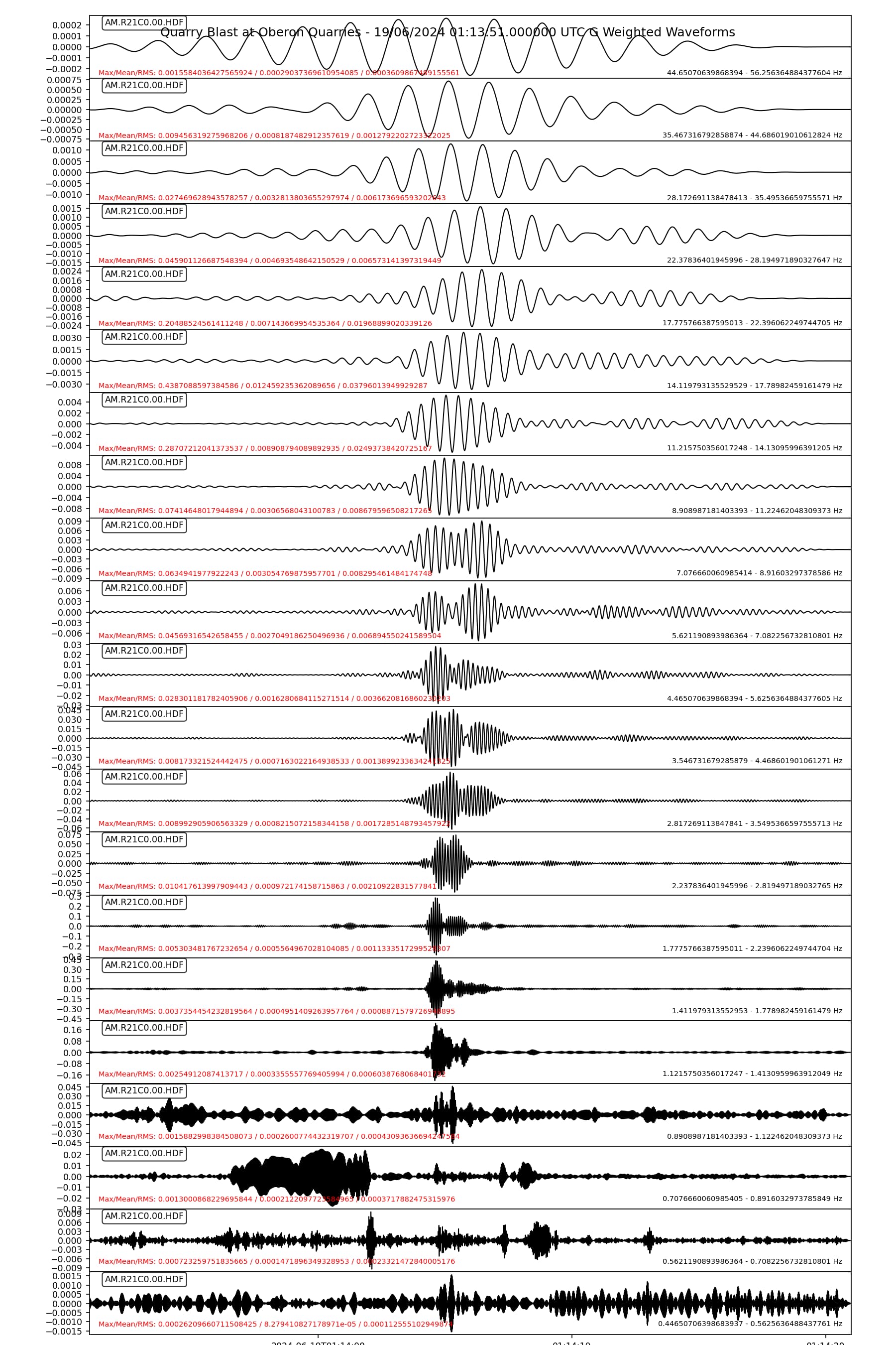
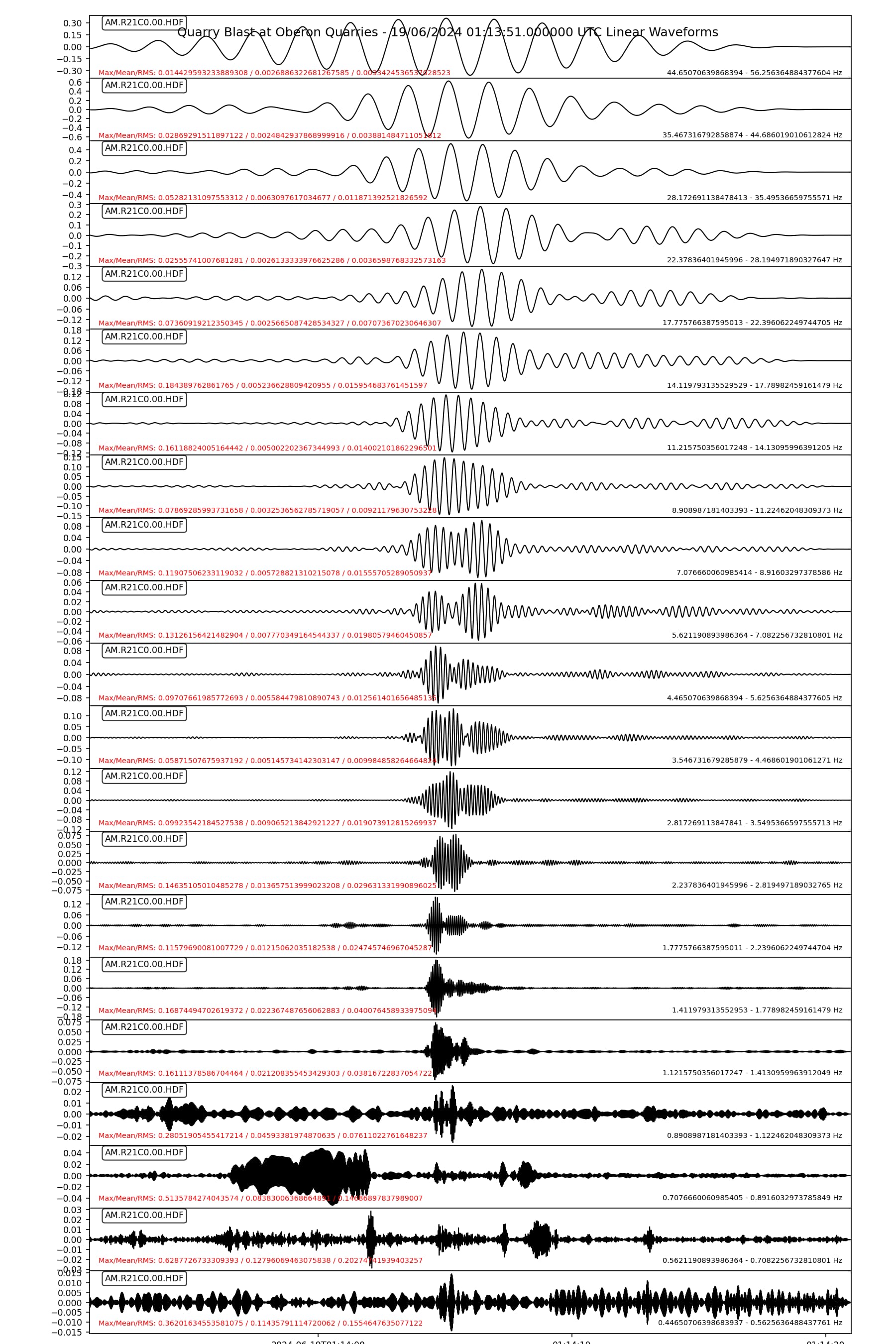
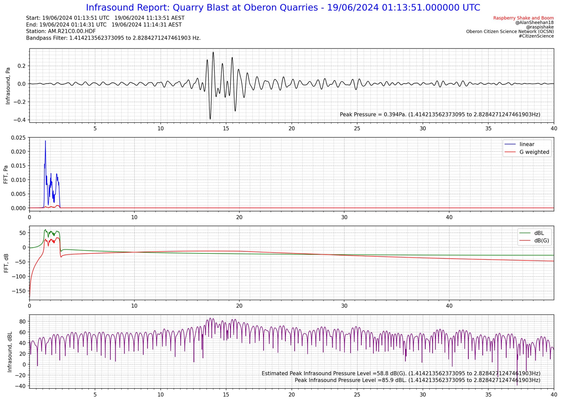
Below are some test plots from the report, which as far as I can find at the moment, it works as it should.
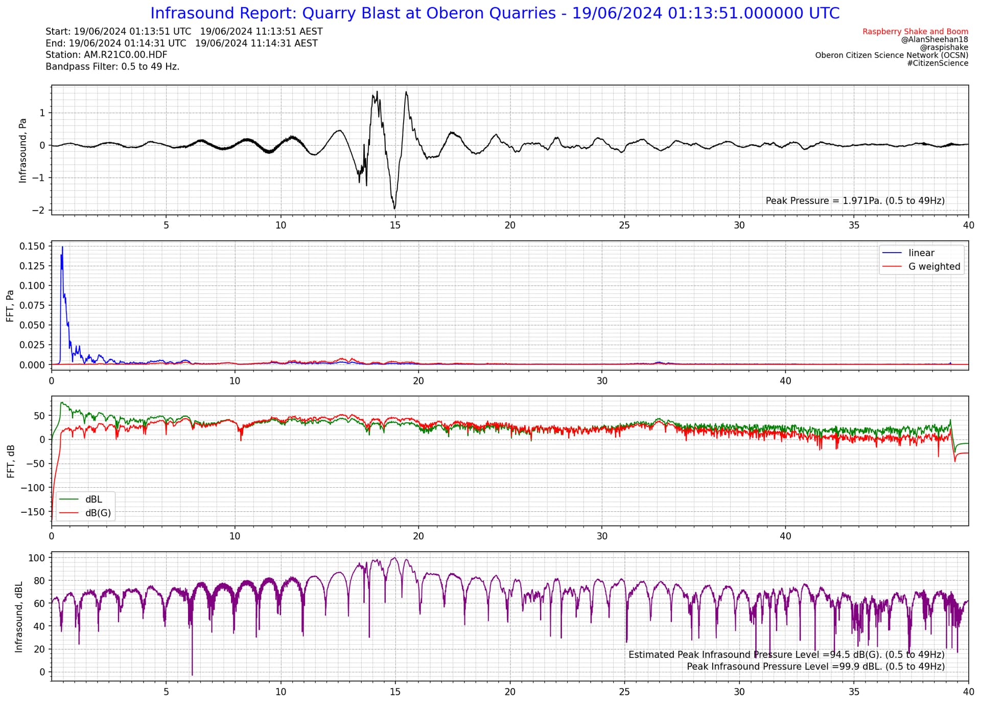
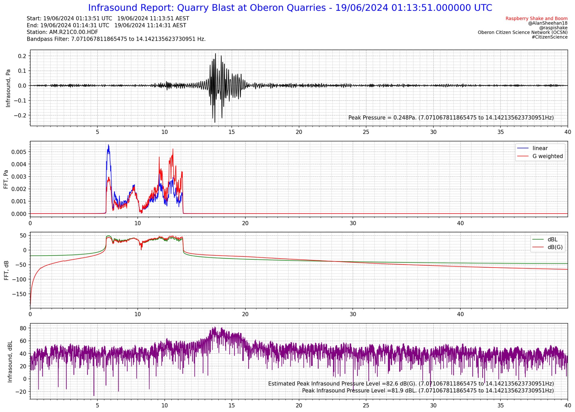
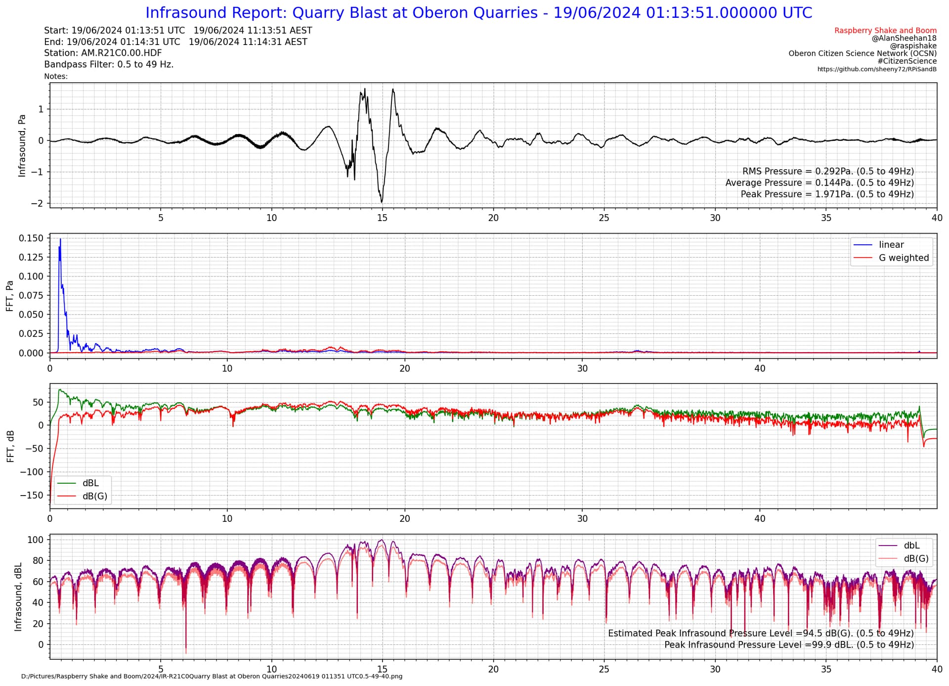
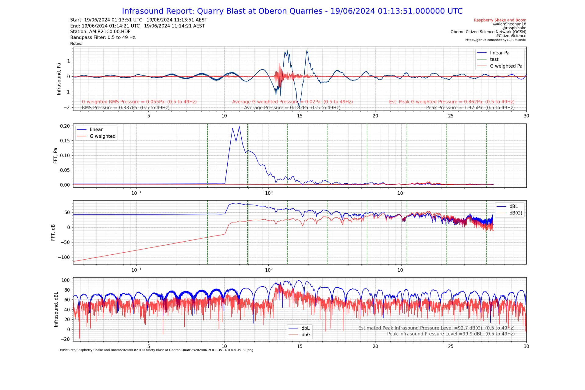
Initial test report, all appears to work as expected. The estimated Peak dB(G) in the time domain is reported in the bottom right corner with the actual peak dBL.
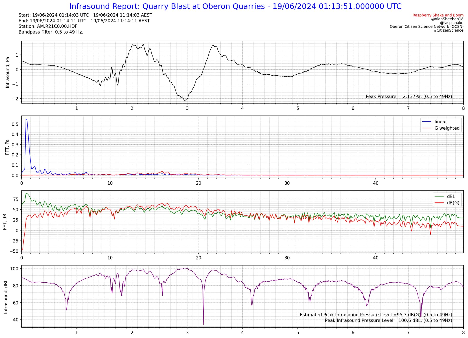
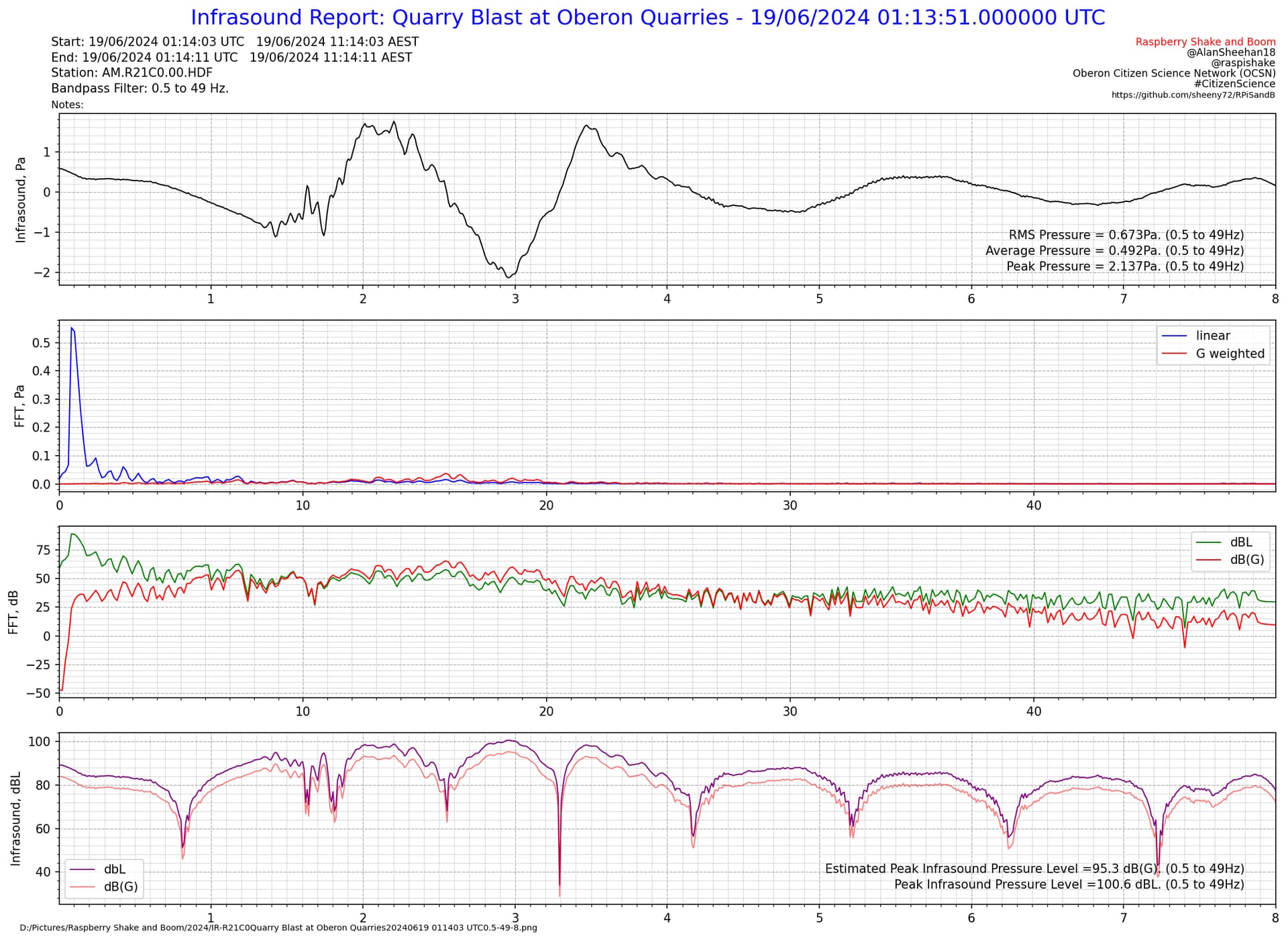
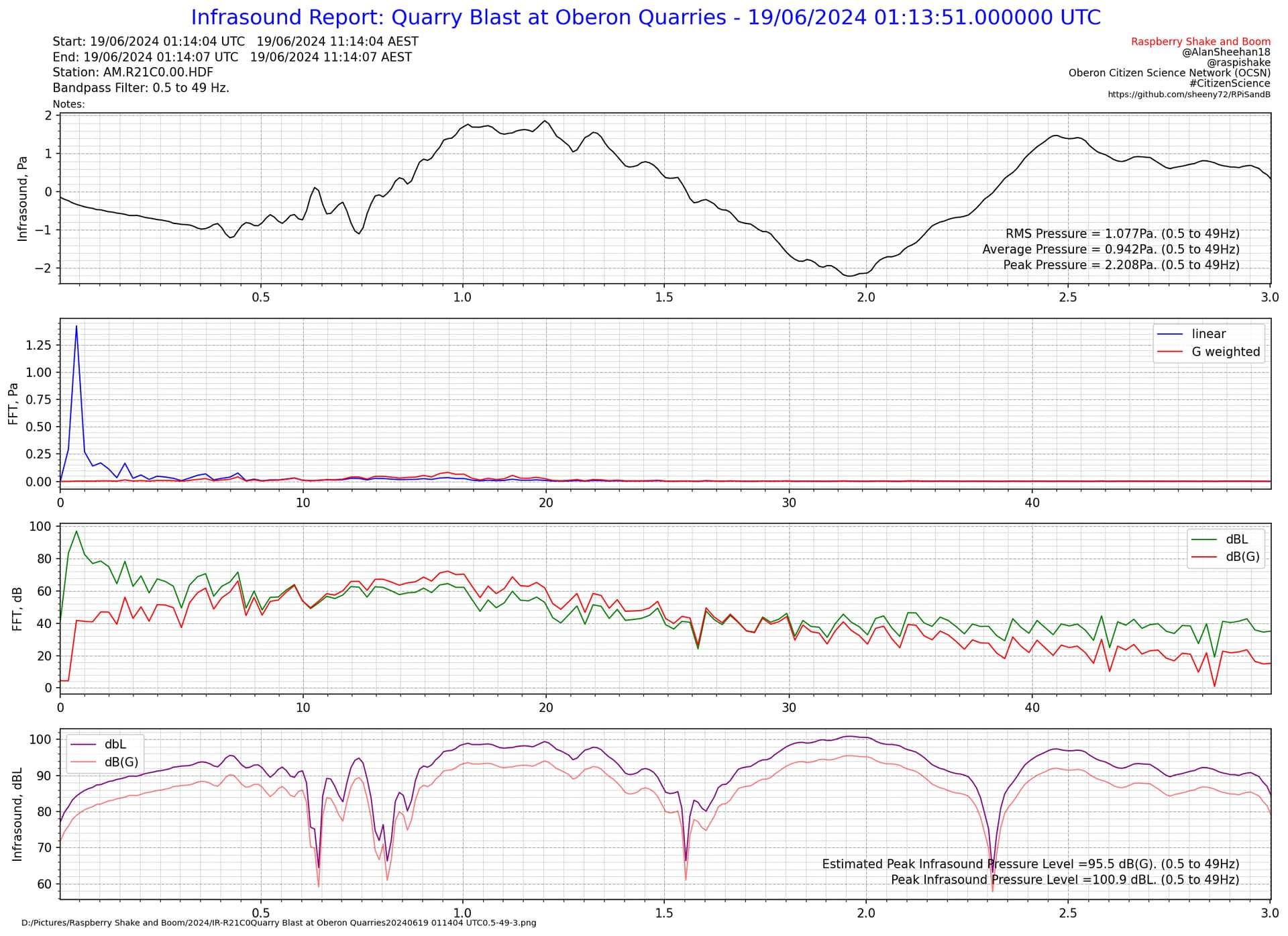
A short duration sample, also seem consistent.
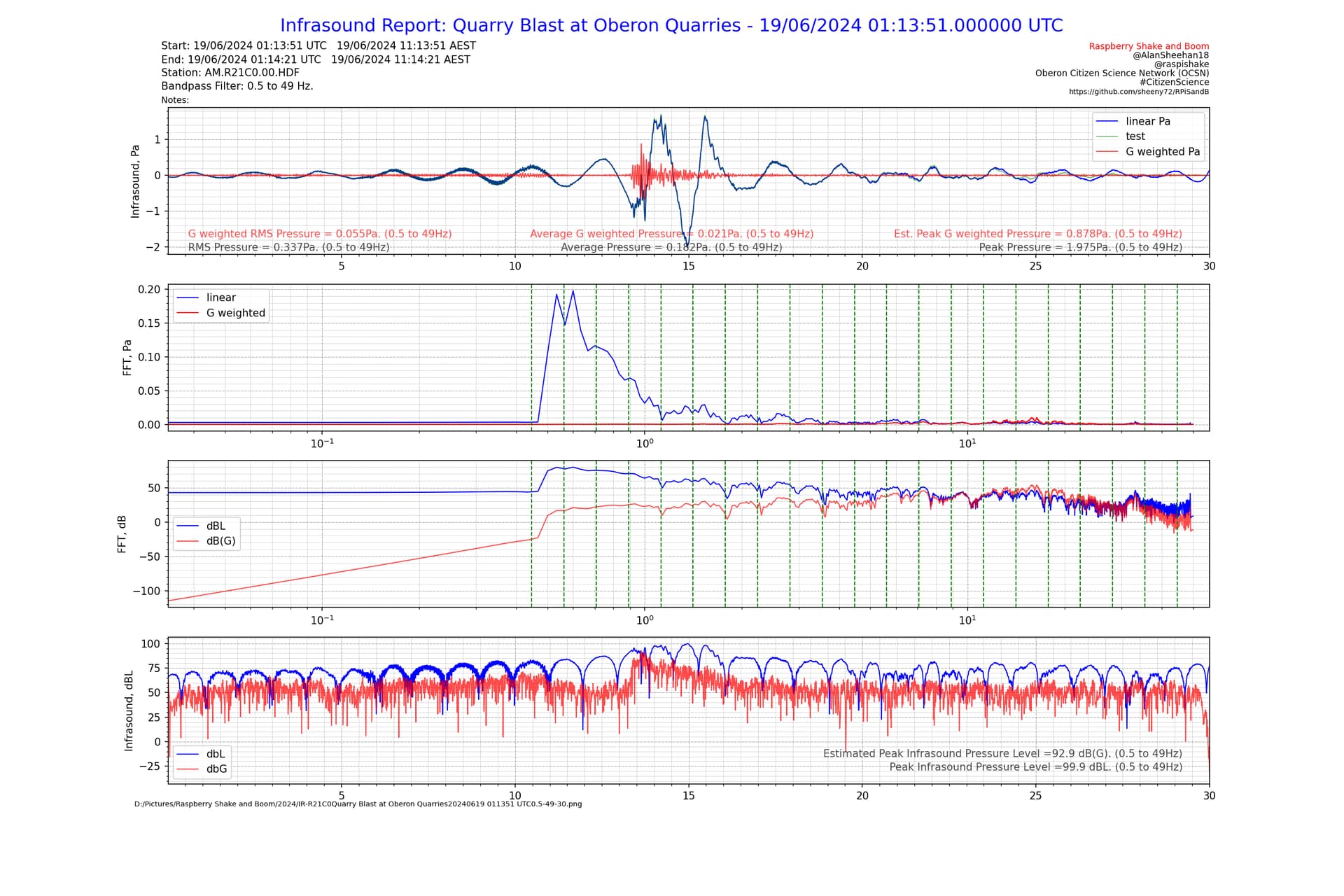
A narrow(er) band test around 10Hz looks as it should as well, and the estimated Peak dB(G) is also behaving as it should. At 10 Hz the G weighting is the same as linear and that shows perfectly.
My initial attempt to estimate the difference between dBL and dB(G) was a result of over thinking the problem. Yes, subtracting dB is the same as division when it is converted back, but it’s valid when using dB!
# -*- coding: utf-8 -*-
"""
Created on Mon Jun 24 08:19:54 2024

@author: al72
"""
from obspy.clients.fdsn import Client
from obspy import UTCDateTime
from matplotlib.ticker import AutoMinorLocator
import numpy as np
import matplotlib.pyplot as plt

# define fdsn client to get data from
client = Client('https://data.raspberryshake.org/')

# define start and end times
eventTime = UTCDateTime(2024, 6, 19, 1, 13, 51) # (YYYY, m, d, H, M, S) **** Enter data****
delay = 0               #delay from event time to start of plot
start = eventTime + delay   #calculate the plot start time
duration = 40               #duration of plot in seconds
end = start + duration                # start plus plot duration in seconds (recommend a minimum of 10s)
daylightSavings = False

# Name the Event
eventName = 'Quarry Blast at Oberon Quarries'       # Name for the Report

# get data from the FSDN server and detrend it
STATION = "R21C0"               # station name
st = client.get_waveforms("AM", STATION, "00", "HDF", starttime=start, endtime=end, attach_response=True)
st.merge(method=0, fill_value='latest')
st.detrend(type="demean")
cmax = abs(st[0].max())     # maximum amplitude of raw counts

# get Instrument Response
inv = client.get_stations(network="AM", station=STATION, level="RESP")

# set up bandpass filter
flc = 0.5      #enter bandpass filter lower corner frequency
fuc = 49        #enter bandpass filter upper corner frequency
filt = [flc-0.01, flc, fuc, fuc+0.1]

# remove instrument response now that raw trace has been processed
y = st.remove_response(inventory=inv,pre_filt=filt,output="DEF", water_level=60)

fs = 100    # sampling frequency
tstep = 1/fs    # sample time interval
f0 = 10     #signal frequency
ns = len(y[0].data)   #number of samples

t = np.linspace(0, (ns-1)*tstep, ns)    # time steps
fstep = fs / ns     # frequency interval
f = np.linspace(0, (ns-1)*fstep, ns)     #frequency steps

# FFT
yfft = np.fft.fft(y[0].data)
y_mag = np.abs(yfft)/ns     #normalise the FFT

f_plot = f[0:int(ns/2+1)]
y_mag_plot = 2*y_mag[0:int(ns/2+1)]
y_mag_plot[0] = y_mag_plot[0]/2     # do not multiply DC value

#calculate maximum sound pressure level
pmax = abs(y[0].max())   #find the max pressure amplitude
splmax = 10*np.log10(pmax*pmax) + 93.979400087        #convert to sound pressure level

# Convert FFT to dB(L)
ydB = []
FFTsum = 0
for i in range (0, len(y_mag_plot.data)):
    ydB.append(20*np.log10(abs(y_mag_plot[i])/0.00002))

# Convert DB(L) to dB(G)
ydBG = []
for i in range (0, len(ydB)):
    if f_plot[i] == 0:
        ydBG.append(ydB[i+1]+34.142*np.log(f_plot[i+1])-41.332)
    elif f_plot[i] < 1:
        ydBG.append(ydB[i]+34.142*np.log(f_plot[i])-41.332)
    elif f_plot[i] <= 3.15:
        ydBG.append(ydB[i]-1.7406*f_plot[i]**4+15.961*f_plot[i]**3-55.565*f_plot[i]**2+95.938*f_plot[i]-97.475)
    elif f_plot[i] < 12.5:
        ydBG.append(ydB[i]+17.396*np.log(f_plot[i])-40.037)
    elif f_plot[i] <= 20:
        ydBG.append(ydB[i]-.0976*f_plot[i]**2+3.8393*f_plot[i]-28.738)
    elif f_plot[i] < 31.5:
        ydBG.append(ydB[i]-.0108*f_plot[i]**2-.5724*f_plot[i]+24.782)
    else:
        ydBG.append(ydB[i]+.0076*f_plot[i]**2-1.4868*f_plot[i]+35.262)

# convert db(G) back to G weighted FFT in Pa
fftG = []
l2G = 0
j = 0
for i in range (0, len(ydB)):
    fftG.append(0.00002*10**(ydBG[i]/20))
    if f_plot[i] >= flc and f_plot[i] < fuc:
        l2G += ydB[i] - ydBG[i]
        j += 1

# estimated Linear to G weighted overall correction
l2G = l2G/j

# plot charts
# set-up figure and subplots
fig = plt.figure(figsize=(18,12), dpi=150)    #18 x 12 inches
ax1 = fig.add_subplot(4,1,1)    #left top 2 high
ax2 = fig.add_subplot(4,1,2)    #left middle 2 high
ax3 = fig.add_subplot(4,1,3)    #right top 2 high
ax4 = fig.add_subplot(4,1,4)    #right middle 2 high
ax1.plot(y[0].times(reftime=start), y[0].data, lw=1, color='k')
ax1.set_ylabel('Infrasound, Pa')
ax1.xaxis.set_minor_locator(AutoMinorLocator(10))
ax1.yaxis.set_minor_locator(AutoMinorLocator(5))
ax1.margins(x=0)
ax2.plot(f_plot, y_mag_plot, lw=1, color = 'b', label='linear')
ax2.plot(f_plot, fftG, lw=1, color = 'r', label='G weighted')
ax2.set_ylabel('FFT, Pa')
ax2.legend()
ax2.xaxis.set_minor_locator(AutoMinorLocator(10))
ax2.yaxis.set_minor_locator(AutoMinorLocator(5))
#ax2.set_yscale('log')
ax2.margins(x=0)
ax3.plot(f_plot, ydB, lw=1, color = 'g', label='dBL')
ax3.set_ylabel('FFT, dB')
ax3.plot(f_plot, ydBG, lw=1, color='r', label='dB(G)')
ax3.legend()
ax3.xaxis.set_minor_locator(AutoMinorLocator(10))
ax3.yaxis.set_minor_locator(AutoMinorLocator(5))
#ax3.set_yscale('log')
ax3.margins(x=0)
ax4.plot(y[0].times(reftime=start), 20*np.log10(abs(y[0].data)/0.00002), lw=1, color='purple')
ax4.set_ylabel('Infrasound, dBL')
ax4.xaxis.set_minor_locator(AutoMinorLocator(10))
ax4.yaxis.set_minor_locator(AutoMinorLocator(5))
ax4.margins(x=0)
ax1.grid(color='dimgray', ls = '-.', lw = 0.33)
ax2.grid(color='dimgray', ls = '-.', lw = 0.33)
ax3.grid(color='dimgray', ls = '-.', lw = 0.33)
ax4.grid(color='dimgray', ls = '-.', lw = 0.33)
ax1.grid(color='dimgray', which='minor', ls = ':', lw = 0.33)
ax2.grid(color='dimgray', which='minor', ls = ':', lw = 0.33)
ax3.grid(color='dimgray', which='minor', ls = ':', lw = 0.33)
ax4.grid(color='dimgray', which='minor', ls = ':', lw = 0.33)

# add text to report
if daylightSavings:
    dsc = 11
    dst = 'AEDT'
else:
    dsc=10
    dst = 'AEST'

fig.suptitle('Infrasound Report: '+eventName+' - '+eventTime.strftime('%d/%m/%Y %H:%M:%S.%f UTC'), size='xx-large',color='b')
fig.text(0.12, 0.945, 'Start: '+start.strftime('%d/%m/%Y %H:%M:%S UTC')+'   '+(start+dsc*3600).strftime('%d/%m/%Y %H:%M:%S '+dst))
fig.text(0.12, 0.93, 'End: '+end.strftime('%d/%m/%Y %H:%M:%S UTC')+'   '+(end+dsc*3600).strftime('%d/%m/%Y %H:%M:%S '+dst))
fig.text(0.12, .915, 'Station: AM.'+STATION+'.00.HDF')
fig.text(0.12, 0.9, 'Bandpass Filter: '+str(flc)+' to '+str(fuc)+' Hz.')
fig.text(0.88, 0.73, 'Peak Pressure = '+str(round(pmax,3))+'Pa. ('+str(filt[1])+" to "+str(filt[2])+"Hz)", ha='right')    #report the peak Pressure
fig.text(0.88, 0.14, 'Peak Infrasound Pressure Level ='+str(round(splmax,1))+' dBL. ('+str(filt[1])+" to "+str(filt[2])+"Hz)", ha='right')   #report peak sound pressure level
fig.text(0.88, 0.155, 'Estimated Peak Infrasound Pressure Level ='+str(round(splmax-l2G,1))+' dB(G). ('+str(filt[1])+" to "+str(filt[2])+"Hz)", ha='right')   #report peak sound pressure level
fig.text(0.9, 0.945, 'Raspberry Shake and Boom', size='small', ha='right', color='r')
fig.text(0.9, 0.935, '@AlanSheehan18', size='small', ha='right')
fig.text(0.9, 0.925, '@raspishake', size='small', ha='right')
fig.text(0.9, 0.915, 'Oberon Citizen Science Network (OCSN)', size='small', ha='right')
fig.text(0.9, 0.905, '#CitizenScience', size='small', ha='right')
Al.