This is my latest coding project: a way to compare the spectra of two waveforms.
The plan was to be able to plot the PSD and/or the FFT from two waveforms on the one graph for clear comparison. This means both sample waveforms need to be the same length. I’ve also constrained the filter frequencies (if used) to be the same on both streams.
Most other things can be changed for the comparison. i.e. different stations, different channels, different outputs (displacement, velocity, acceleration, or Infrasound Pressure), raw counts or filtered units. Not all combinations of comparison units are necessarily meaningful, but may serve, say, an education purpose. For example, compare the same sample time and station and channel in both velocity and acceleration to show the bias towards higher frequencies when using acceleration output.
My main reason for doing this is to explore what frequencies are produced by some events, particularly with a Boom: lightning, wind, rain, etc.
Apart from displaying the PSD and FFT of two sample waveforms on the same graph, why not plot the differences? So I had a go at that as well for the FFT differences, but it turns out to not be as simple as it would appear at first thought. Somewhere in the FFT process complex numbers appear, so simple arithmetic subtraction of one FFT plot from another produces a warning that the complex component is being ignored.
I’ve come up with three ways to calculate the FFT difference (I suspect there are more - at least 1 for sure). At this stage, I don’t know which if any method is correct/valid but interestingly they are all consistent regardless of whether sample 1 is subtracted from sample 2 or vice versa. If anyone with some experience or understanding of FFT signal procressing can offer any constructive critcism on which method is valid, this would be greatly appreciated. For now, I’m plotting all three methods that I’ve coded.
Another query someone may be able to help with is how to subtract a PSD from another PSD. It’s not immediately obvious if this is possible the way the PSD’s are handled in Obspy.
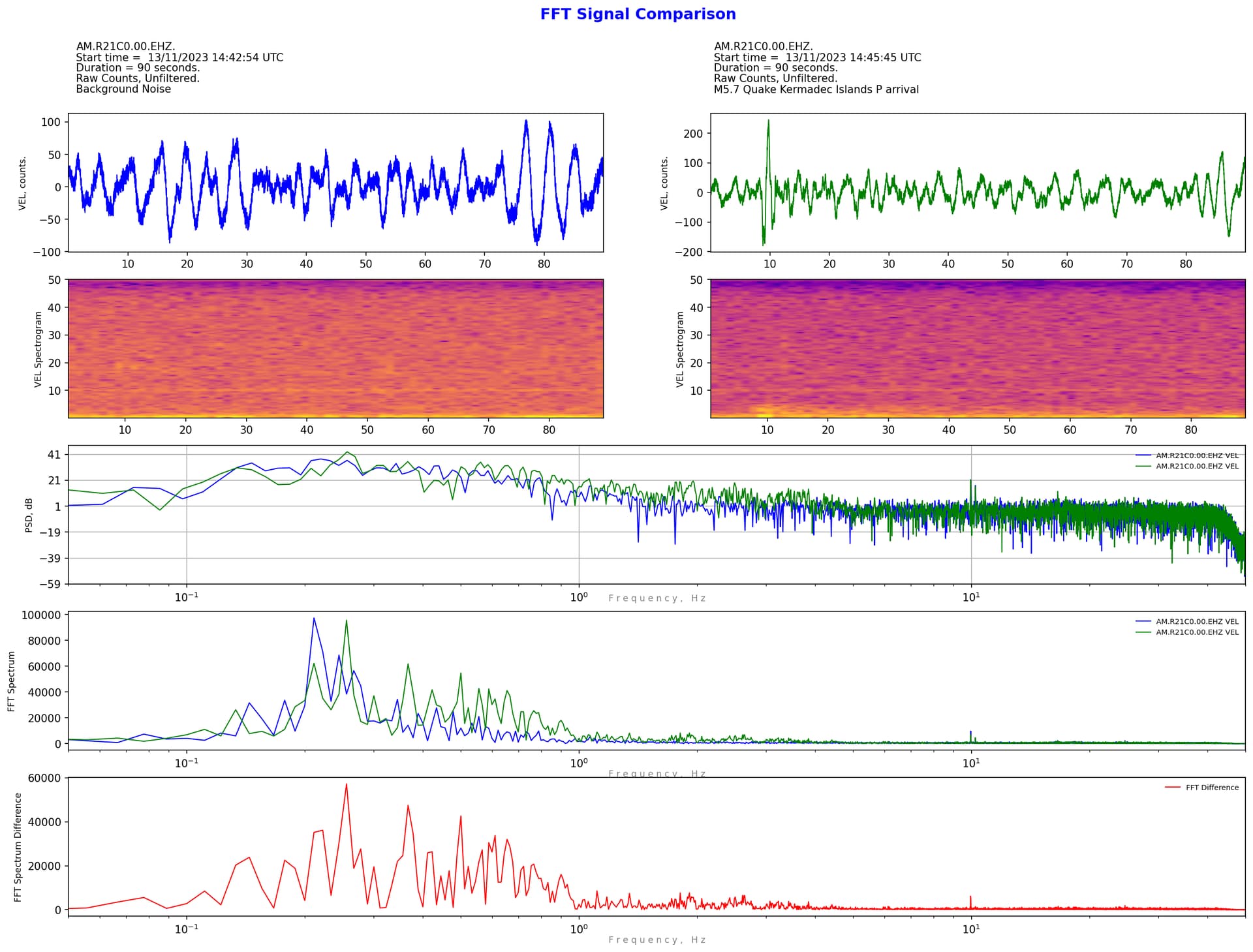
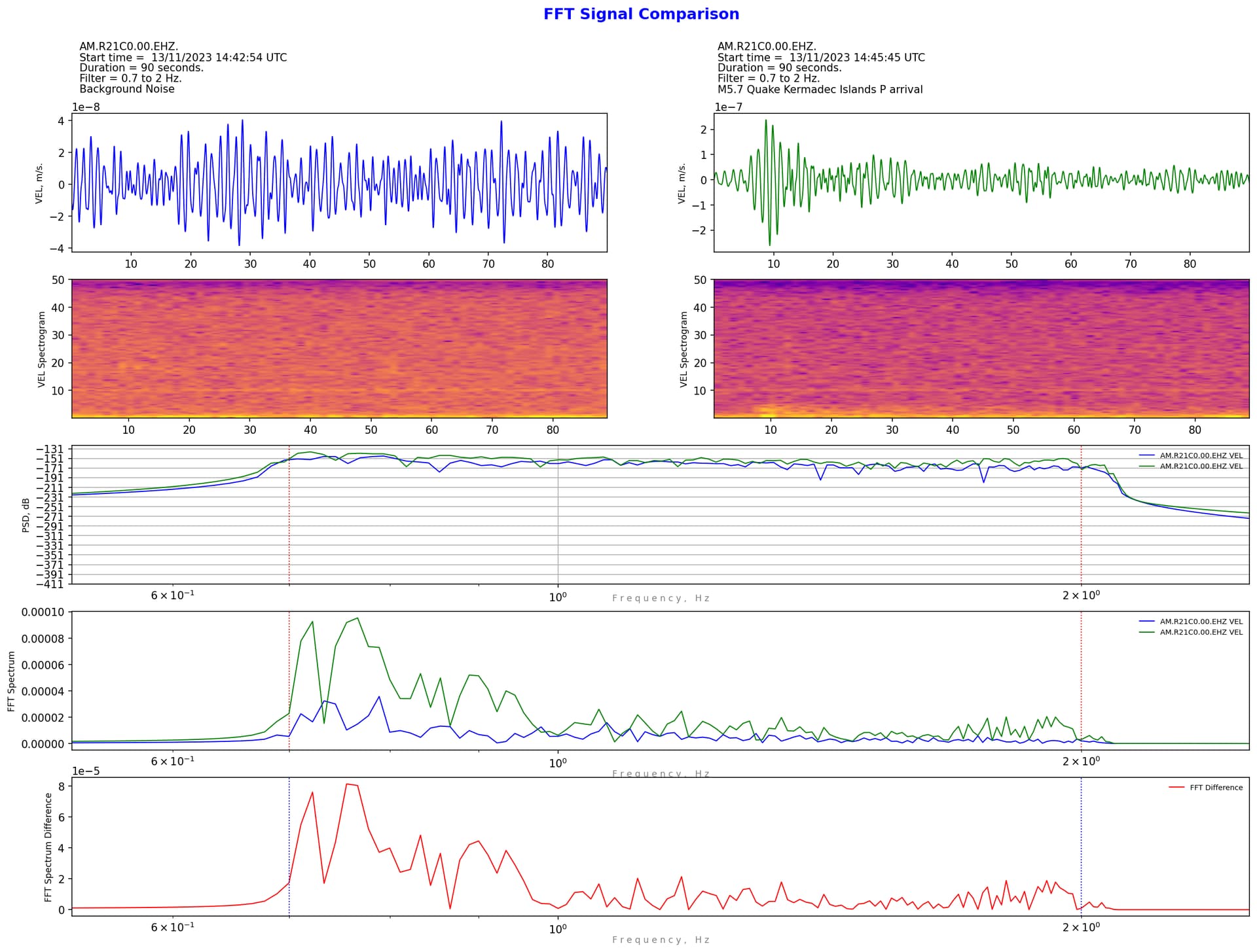
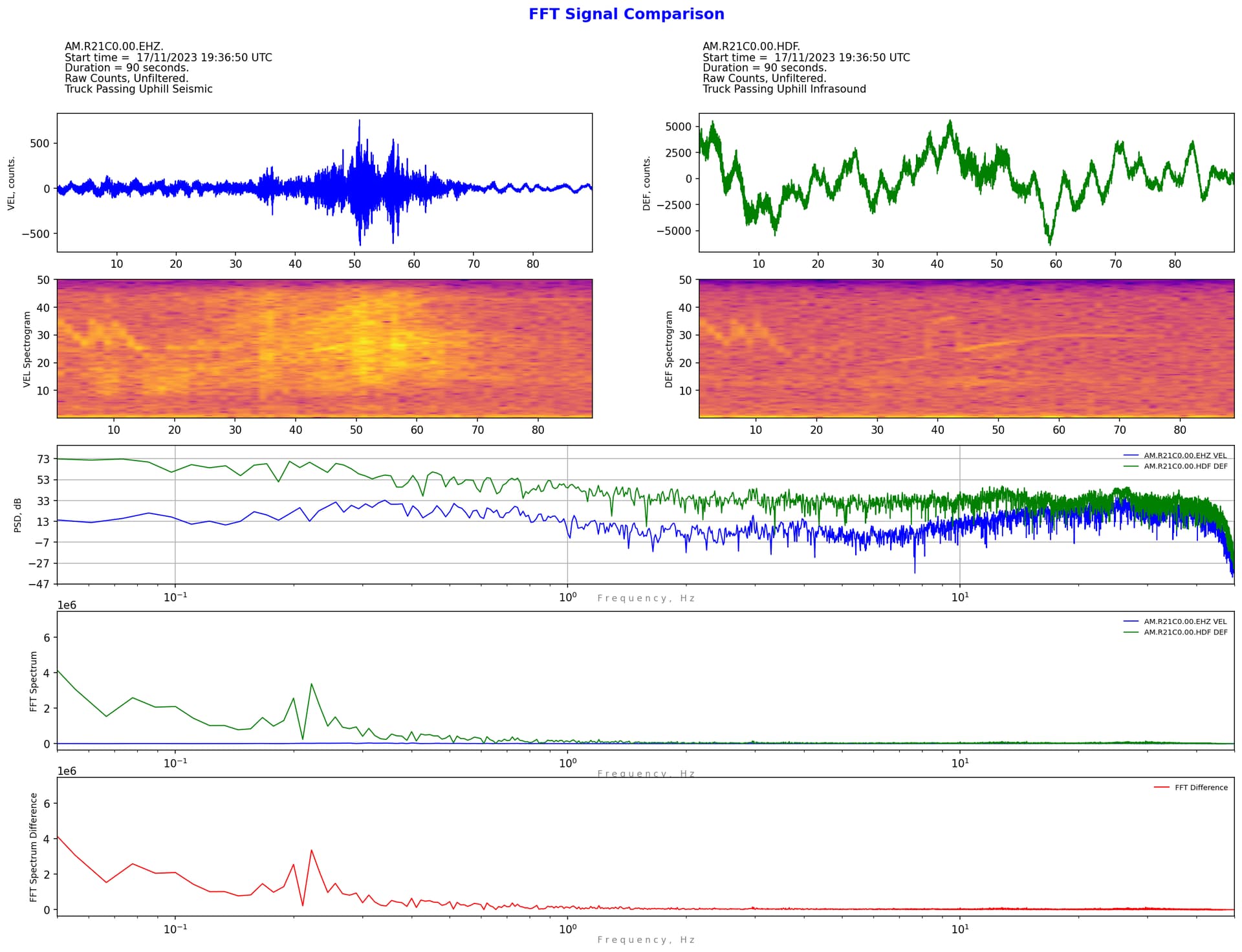
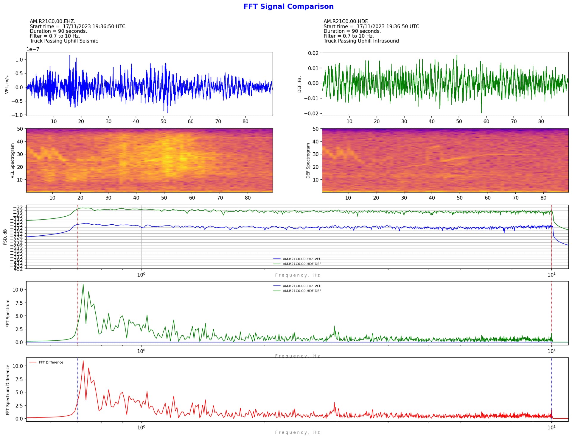
Anyway, FWIW here is a first example of the output from the code. This is comparision of the arrival of the P wave from the M5.7 Kermedec Islands Quake with background noise just before the arrival:
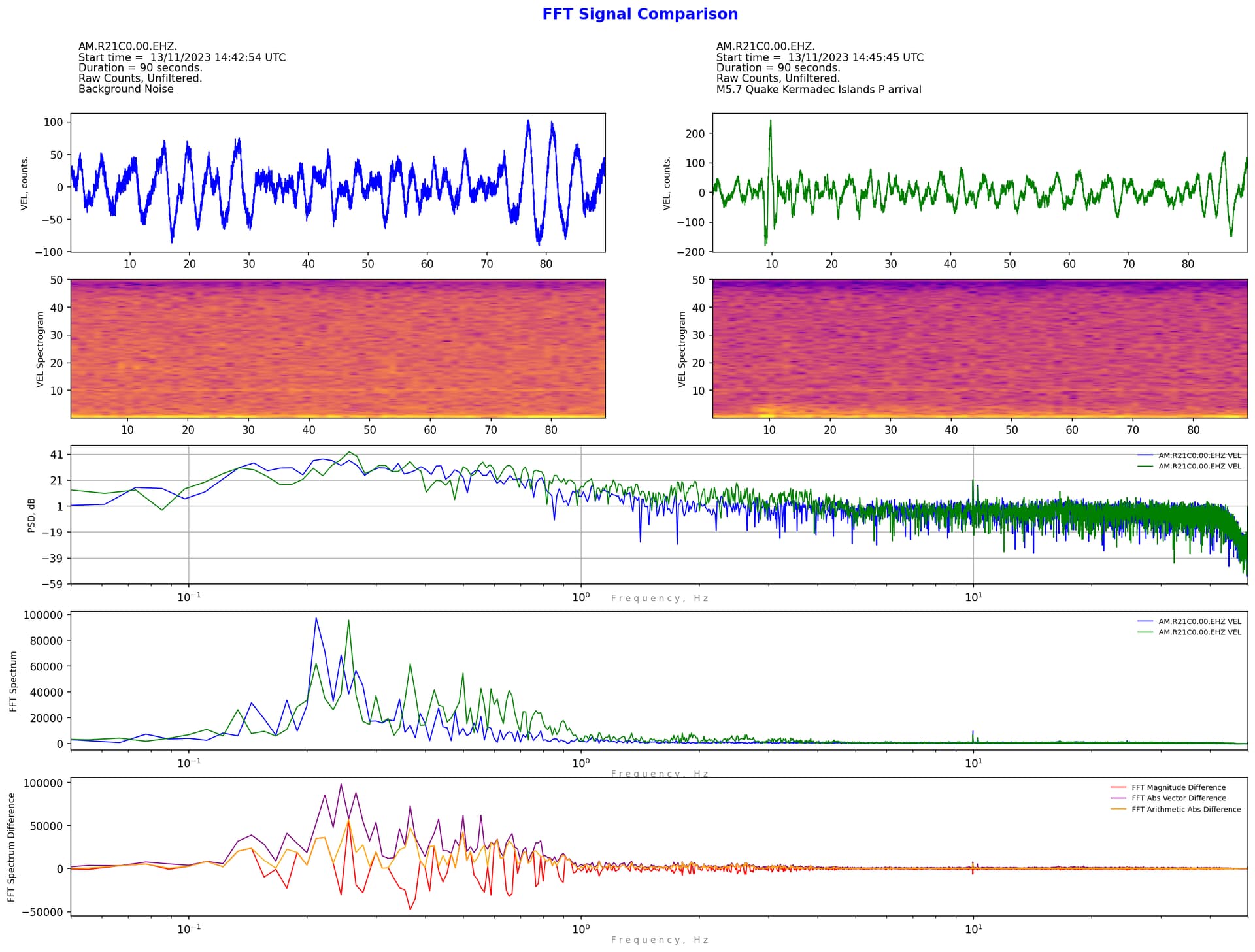
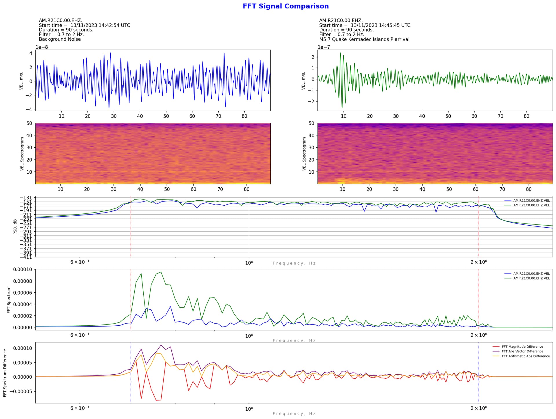
As you can see, after comparing the raw counts, it is possible to apply a filter to both samples and hence “zoom in” to whatever areas of the frequency spectrum is of interest.
Here is the code so far. Probably not the tidiest, but happy for anyone to use and play with it and modify as they see fit.
# -*- coding: utf-8 -*-
"""
Created on Thu Nov 16 10:52:26 2023

@author: al72
"""

# Spectrum comparison for the Raspberry Shake and Boom

from obspy.clients.fdsn import Client
from obspy.core import UTCDateTime
import matplotlib.pyplot as plt
import numpy as np


rs = Client('https://data.raspberryshake.org/')

def FFTsub(f1, f2):
    n = len(f1)
    diff = []
    for i in range(0,n):
        if f1[i] >= f2[i]:
            diff.append(abs(f1[i]) - abs(f2[i]))
        else:
            diff.append(abs(f2[i]) - abs(f1[i]))
    return diff

# Channel 1 data
startTime1 = UTCDateTime(2023, 11, 13, 14, 42, 54) # (YYYY, m, d, H, M, S) **** Enter data****

# set the station name and download the response information
stn1 = 'R21C0'      # station name
nw1 = 'AM'          # network name
#ch1 = ['EHZ', 'DISP', 'm.']
ch1 = ['EHZ', 'VEL', 'm/s.']
#ch1 = ['EHZ', 'ACC', 'm/s².']
#ch1 = ['HDF', 'DEF', 'Pa.']
inv1 = rs.get_stations(network=nw1, station=stn1, level='RESP')  # get the instrument response
notes1 = 'Background Noise'

# Channel 2 data
startTime2 = UTCDateTime(2023, 11, 13, 14, 45, 45) # (YYYY, m, d, H, M, S) **** Enter data****

# set the station name and download the response information
stn2 = 'R21C0'      # station name
nw2 = 'AM'          # network name
#ch2 = ['EHZ', 'DISP', 'm.']
ch2 = ['EHZ', 'VEL', 'm/s.']
#ch2 = ['EHZ', 'ACC', 'm/s².']
#ch2 = ['HDF', 'DEF', 'Pa.']
inv2 = rs.get_stations(network=nw2, station=stn2, level='RESP')  # get the instrument response
notes2 = 'M5.7 Quake Kermadec Islands P arrival'

#Setup the data plot
duration = 90               # duration of plots in seconds **** Enter data****
end1 = startTime1 + duration
end2 = startTime2 + duration
filtered = True
logspect = False
filt = [0.69, 0.7, 2, 2.1]

# calculate spectrum plot limits if filtered
if filtered:
    if filt[2] >=4:
        fxt = filt[2]+1
    else:
        fxt = filt[2]*1.25
    if filt[1] >= 2:
        fxb = filt[1]-1
    else:
        fxb = filt[1]*0.75
else:
    fxt = 50
    fxb = 0.05

# get and process the waveforms
trace1 = rs.get_waveforms(nw1, stn1, '00', ch1[0], startTime1, end1)
trace1.merge(method=0, fill_value='latest')         #fill in any gaps in the data to prevent a crash
trace1.detrend(type='demean')                       #demean the data
raw1 = trace1.copy()
trace1.remove_response(inventory=inv1,pre_filt=filt,output=ch1[1],water_level=60, plot=False)

trace2 = rs.get_waveforms(nw2, stn2, '00', ch2[0], startTime2, end2)
trace2.merge(method=0, fill_value='latest')         #fill in any gaps in the data to prevent a crash
trace2.detrend(type='demean')                       #demean the data
raw2 = trace2.copy()
trace2.remove_response(inventory=inv2,pre_filt=filt,output=ch2[1],water_level=60, plot=False)

# set up plot
fig = plt.figure(figsize=(20,14), dpi=150)       # set to page size in inches
ax1 = fig.add_subplot(5, 2, 1)      # waveform 1 plot
ax2 = fig.add_subplot(5, 2, 2)      # waveform 2 plot
ax3 = fig.add_subplot(5, 2, 3)      # waveform 1 spectrogram
ax4 = fig.add_subplot(5, 2, 4)      # waveform 2 spectrogram
ax5 = fig.add_subplot(5, 2, (5,6))      # PSD plots
ax6 = fig.add_subplot(5, 2, (7,8))      # FFT plots
ax7 = fig.add_subplot(5, 2, (9,10))     # FFT difference plots

#plot traces
if filtered:
    ax1.plot(trace1[0].times(reftime=startTime1), trace1[0].data, lw=1, color='b')      # displacement waveform
    ax2.plot(trace2[0].times(reftime=startTime2), trace2[0].data, lw=1, color='g')
    ax1.set_ylabel(ch1[1]+', '+ch1[2],size='small')
    ax2.set_ylabel(ch2[1]+', '+ch2[2],size='small')
else:
    ax1.plot(raw1[0].times(reftime=startTime1), raw1[0].data, lw=1, color='b')      # displacement waveform
    ax2.plot(raw2[0].times(reftime=startTime2), raw2[0].data, lw=1, color='g')
    ax1.set_ylabel(ch1[1]+', counts.',size='small')
    ax2.set_ylabel(ch2[1]+', counts.',size='small')
ax1.margins(x=0)
ax2.margins(x=0)

ax3.specgram(x=raw1[0], NFFT=256, noverlap=128, Fs=100, cmap='plasma')         # velocity spectrogram
ax3.set_ylabel(ch1[1]+' Spectrogram',size='small')
if logspect:
    ax3.set_yscale('log')
ax3.set_ylim(0.05, 50)
ax4.specgram(x=raw2[0], NFFT=256, noverlap=128, Fs=100, cmap='plasma')         # velocity spectrogram
ax4.set_ylabel(ch2[1]+' Spectrogram',size='small')
if logspect:
    ax4.set_yscale('log')
ax4.set_ylim(0.05, 50)

#plot PSD
#calculate NFFT for PSD
if duration >= 82:
    nfft = 8192
else:
    nfft = duration*100
if filtered:
    ax5.psd(x=trace1[0], NFFT=nfft, noverlap=0, Fs=100, color='b', lw=1, label=nw1+'.'+stn1+'.00.'+ch1[0]+' '+ch1[1])
    ax5.psd(x=trace2[0], NFFT=nfft, noverlap=0, Fs=100, color='g', lw=1, label=nw2+'.'+stn2+'.00.'+ch2[0]+' '+ch2[1])
    #plot filter limits on PSD
    ax5.axvline(x=filt[1], linewidth=1, linestyle='dotted', color='r')
    ax5.axvline(x=filt[2], linewidth=1, linestyle='dotted', color='r')
else:
    ax5.psd(x=raw1[0], NFFT=nfft, noverlap=0, Fs=100, color='b', lw=1, label=nw1+'.'+stn1+'.00.'+ch1[0]+' '+ch1[1])
    ax5.psd(x=raw2[0], NFFT=nfft, noverlap=0, Fs=100, color='g', lw=1, label=nw2+'.'+stn2+'.00.'+ch2[0]+' '+ch2[1])
ax5.set_xlim(fxb, fxt)
#ax5.set_ylim(-290, -130)
ax5.legend(frameon=False, fontsize='x-small')
ax5.set_xscale('log')               #use logarithmic scale on PSD
#ax5.set_yscale('linear')
#ax5.set_yscale('log')
ax5.set_ylabel("PSD, dB",size='small')
ax5.set_xlabel('F r e q u e n c y ,   H z', size='small', alpha=0.5, labelpad=-9)


# fourier analysis plot
if filtered:
    fft1 = np.fft.rfft(trace1[0].data)
    fft2 = np.fft.rfft(trace2[0].data)
    xfft = np.fft.rfftfreq(trace1[0].data.size, d = 1/100)
    # plot filter limits on FFT
    ax6.axvline(x=filt[1], linewidth=1, linestyle='dotted', color='r')
    ax6.axvline(x=filt[2], linewidth=1, linestyle='dotted', color='r')
else:
    fft1 = np.fft.rfft(raw1[0].data)
    fft2 = np.fft.rfft(raw2[0].data)
    xfft = np.fft.rfftfreq(raw1[0].data.size, d = 1/100)
ax6.set_xlim(fxb, fxt)
ax6.plot(xfft, abs(fft1), color='b', lw=1, label=nw1+'.'+stn1+'.00.'+ch1[0]+' '+ch1[1])
ax6.plot(xfft, abs(fft2), color='g', lw=1, label=nw2+'.'+stn2+'.00.'+ch2[0]+' '+ch2[1])
ax6.legend(frameon=False, fontsize='x-small')
ax6.set_xscale('log')               #use logarithmic scale on FFT
#ax6.set_yscale('linear')
#ax6.set_yscale('log')
ax6.set_ylabel("FFT Spectrum",size='small')
ax6.set_xlabel('F r e q u e n c y ,   H z', size='small', alpha=0.5, labelpad=0)

# fourier difference plot
dfft = FFTsub(fft1, fft2)
dfft1 = fft1 - fft2
dfft2 = abs(fft1) - abs(fft2)
ax7.plot(xfft, dfft, color='r', lw=1, label='FFT Magnitude Difference')
ax7.plot(xfft, abs(dfft1), color='purple', lw=1, label='FFT Abs Vector Difference')
ax7.plot(xfft, abs(dfft2), color='orange', lw=1, label='FFT Arithmetic Abs Difference')
ax7.legend(frameon=False, fontsize='x-small')
ax7.margins(x=0)
if filtered:
    ax7.axvline(x=filt[1], linewidth=1, linestyle='dotted', color='b')
    ax7.axvline(x=filt[2], linewidth=1, linestyle='dotted', color='b')
ax7.set_xlim(fxb, fxt)
ax7.set_xscale('log')               #use logarithmic scale on FFT Difference
ax7.set_ylabel("FFT Spectrum Difference",size='small')
ax7.set_xlabel('F r e q u e n c y ,   H z', size='small', alpha=0.5, labelpad=0)

fig.suptitle("FFT Signal Comparison", weight='black', color='b', size='x-large')      #Title of the figure
fig.text(0.13, 0.94, nw1+'.'+stn1+'.00.'+ch1[0]+'.')
fig.text(0.13, 0.93, 'Start time = '+startTime1.strftime(' %d/%m/%Y %H:%M:%S UTC'))
fig.text(0.13, 0.92, 'Duration = '+str(duration)+' seconds.')
if filtered:
    fig.text(0.13, 0.91, 'Filter = '+str(filt[1])+' to '+str(filt[2])+' Hz.')
else:
    fig.text(0.13, 0.91, 'Raw Counts, Unfiltered.')
fig.text(0.13, 0.9, notes1)

fig.text(0.55, 0.94, nw2+'.'+stn2+'.00.'+ch2[0]+'.')
fig.text(0.55, 0.93, 'Start time = '+startTime2.strftime(' %d/%m/%Y %H:%M:%S UTC'))
fig.text(0.55, 0.92, 'Duration = '+str(duration)+' seconds.')
if filtered:
    fig.text(0.55, 0.91, 'Filter = '+str(filt[1])+' to '+str(filt[2])+' Hz.')
else:
    fig.text(0.55, 0.91, 'Raw Counts, Unfiltered.')
fig.text(0.55, 0.9, notes2)