I have noticed timeouts occurring over the last few days and they seem to be getting more frequent. I assume this could be a server problem but if it’s something my end that I can fix I’d like to know?
Thanks,
Al.
I have noticed timeouts occurring over the last few days and they seem to be getting more frequent. I assume this could be a server problem but if it’s something my end that I can fix I’d like to know?
Thanks,
Al.
Hello Sheeny,
Could you post the code (or the portion of the code) that generates this issue so we can try to re-create it here?
Thank you!
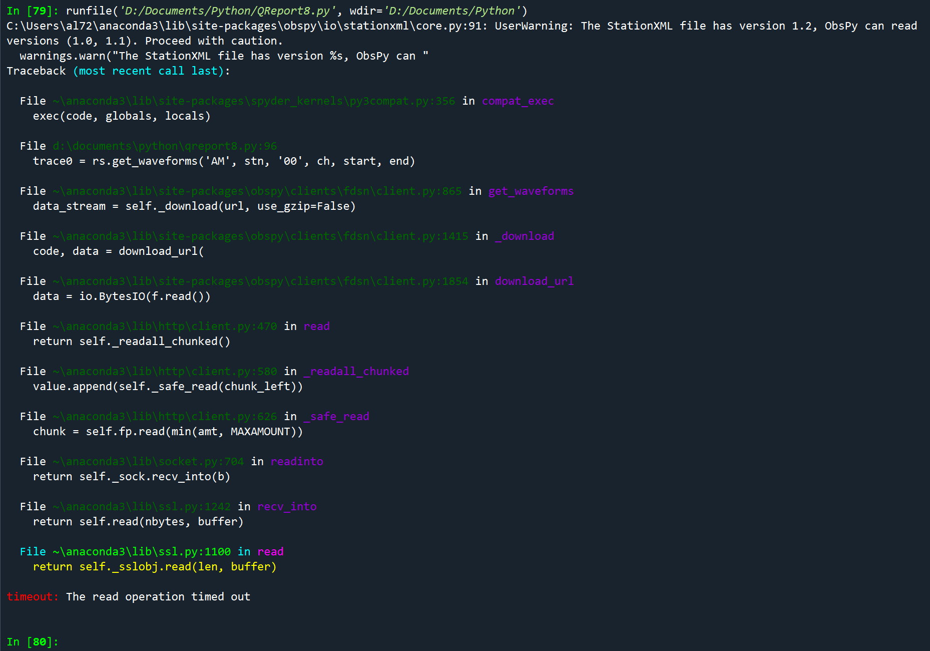
Sure. Here’s the full code:
from obspy.clients.fdsn import Client
from obspy.core import UTCDateTime
from obspy.signal import filter
import matplotlib.pyplot as plt
from matplotlib.ticker import AutoMinorLocator
import numpy as np
from obspy.taup import TauPyModel
import math
import cartopy.crs as ccrs
import cartopy.feature as cfeature
rs = Client('https://data.raspberryshake.org/')
def plot_arrivals(ax, d1):
y1 = -1
axb, axt = ax.get_ylim() # calculate the y limits of the graph
for q in range(0, no_arrs): #plot each arrival in turn
x1 = arrs[q].time # extract the time to plot
if (x1 >= delay):
if x1 < delay+duration:
ax.axvline(x=x1-d1, linewidth=0.5, linestyle='--', color='black') # draw a vertical line
if y1 < 0 or y1 < axt/2: # alternate top and bottom for phase tags
y1 = axt*0.8
else:
y1 = axb*0.95
ax.text(x1-d1,y1,arrs[q].name, alpha=0.5) # print the phase name
x1 = rayt #plot the Rayleight Surface Wave arrival
if (x1>=delay):
if x1 < delay+duration:
ax.axvline(x=x1-d1, linewidth=0.5, linestyle='--', color='black') # draw a vertical line
if y1 < 0 or y1 < axt/2: # alternate top and bottom for phase tags
y1 = axt*0.8
else:
y1 = axb*0.95
ax.text(x1-d1,y1,'Ray', alpha=0.5) # print the phase name
def time2UTC(a): #convert time (seconds) since event back to UTCDateTime
return eventTime + a
def uTC2time(a): #convert UTCDateTime to seconds since the event
return a - eventTime
def one_over(a): # 1/x to convert frequency to period
#Vectorized 1/a, treating a==0 manually
a = np.array(a).astype(float)
near_zero = np.isclose(a, 0)
a[near_zero] = np.inf
a[~near_zero] = 1 / a[~near_zero]
return a
inverse = one_over #function 1/x is its own inverse
def plot_noiselims(ax, uplim, downlim):
axl, axr = ax.get_xlim()
ax.axhline(y=uplim, lw=0.33, color='r', linestyle='dotted') #plot +1 SD
ax.axhline(y=uplim*2, lw=0.33, color='r', linestyle='dotted') #plot +2 SD
ax.axhline(y=uplim*3, lw=0.33, color='r', linestyle='dotted') #plot upper background noise limit +3SD
ax.axhline(y=downlim, lw=0.33, color='r', linestyle='dotted') #plot -1 SD
ax.axhline(y=downlim*2, lw=0.33, color='r', linestyle='dotted') #plot -2SD
ax.axhline(y=downlim*3, lw=0.33, color='r', linestyle='dotted') #plot lower background noise limit -3SD
ax.text(axl, uplim*3,'3SD background', size='xx-small', color='r',alpha=0.5, ha='left', va='bottom')
ax.text(axl, downlim*3, '-3SD background', size='xx-small', color='r', alpha=0.5, ha='left', va='top')
def plot_se_noiselims(ax, uplim):
axl, axr = ax.get_xlim()
ax.axhline(y=uplim, lw=0.33, color='r', linestyle='dotted') #plot +1 SD
ax.axhline(y=uplim*2*2, lw=0.33, color='r', linestyle='dotted') #plot +2 SD
ax.axhline(y=uplim*3*3, lw=0.33, color='r', linestyle='dotted') #plot upper background noise limit +3SD
ax.axhline(y=0, lw=0.33, color='r', linestyle='dotted') #plot 0 limit in case data has no zero
ax.text(axl, uplim*3*3,'3SD background', size='xx-small', color='r',alpha=0.5, ha='left', va='bottom')
def divTrace(tr, n): #divide trace into n equal parts for background noise determination
return tr.__div__(n)
def fmtax(ax, lim, noneg): #pass axis, 0 for auto y scaling or manual limit, True if no negatives in plot i.e. Specific energy
ax.xaxis.set_minor_locator(AutoMinorLocator(10))
ax.yaxis.set_minor_locator(AutoMinorLocator(5))
ax.set_xlabel('Seconds after Event, s', size='small', labelpad=0)
grid(ax)
if lim!=0:
if noneg:
ax.set_ylim(0, lim)
else:
ax.set_ylim(-lim, lim) # set manual y limits for displacement- comment this out for autoscaling
def grid(ax): #pass axis
ax.grid(color='dimgray', ls = '-.', lw = 0.33)
ax.grid(color='dimgray', which='minor', ls = ':', lw = 0.33)
def sax(secax, tix): #pass secondary axis, and ticks
secax.set_xticks(ticks=tix)
secax.set_xticklabels(tlabels, size='small', va='center_baseline')
secax.xaxis.set_minor_locator(AutoMinorLocator(10))
# set the station name and download the response information
stn = 'R21C0' # your station name
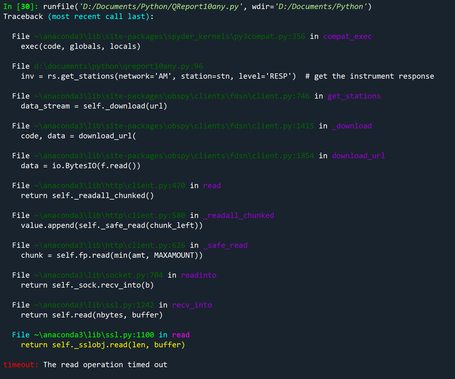
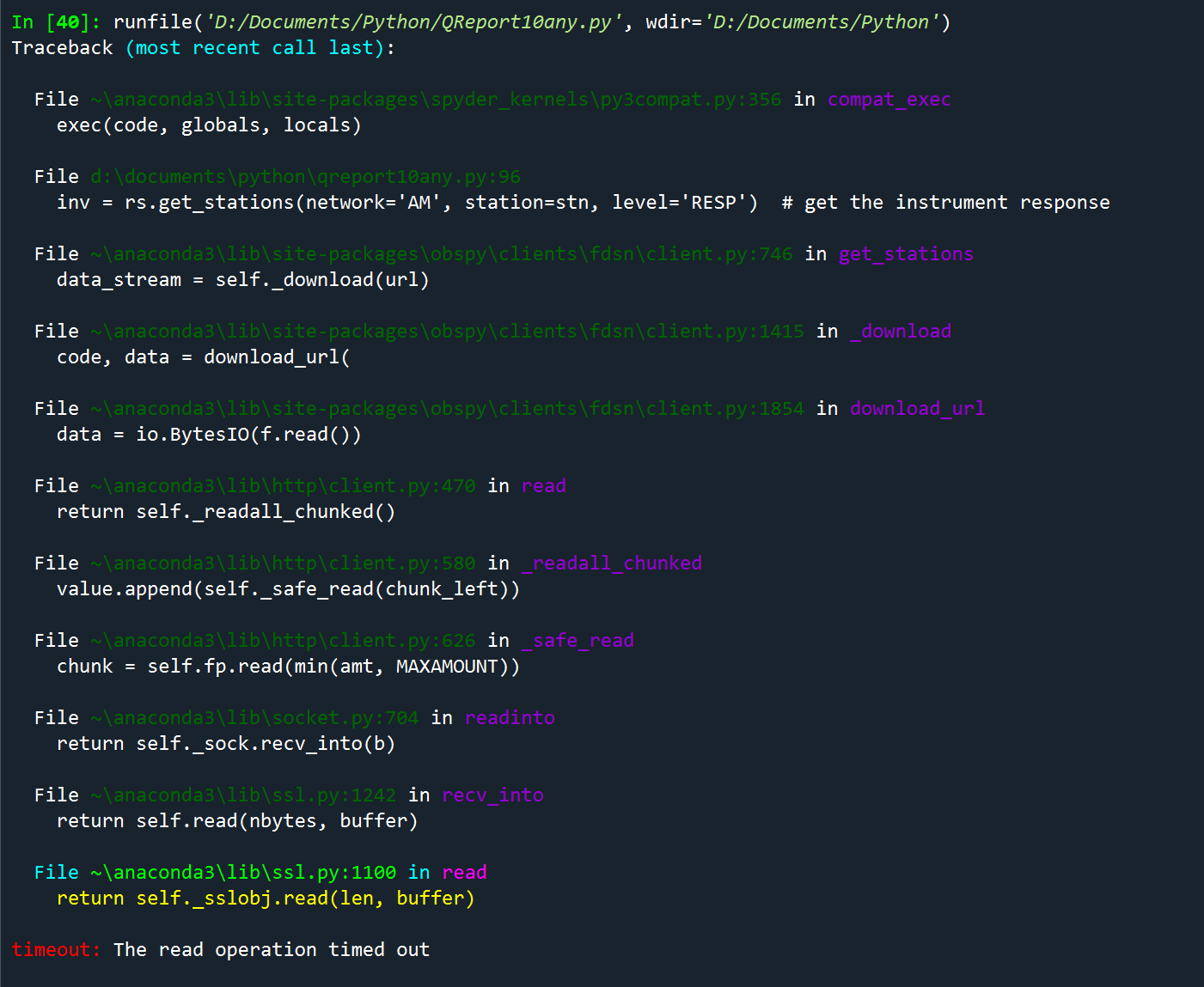
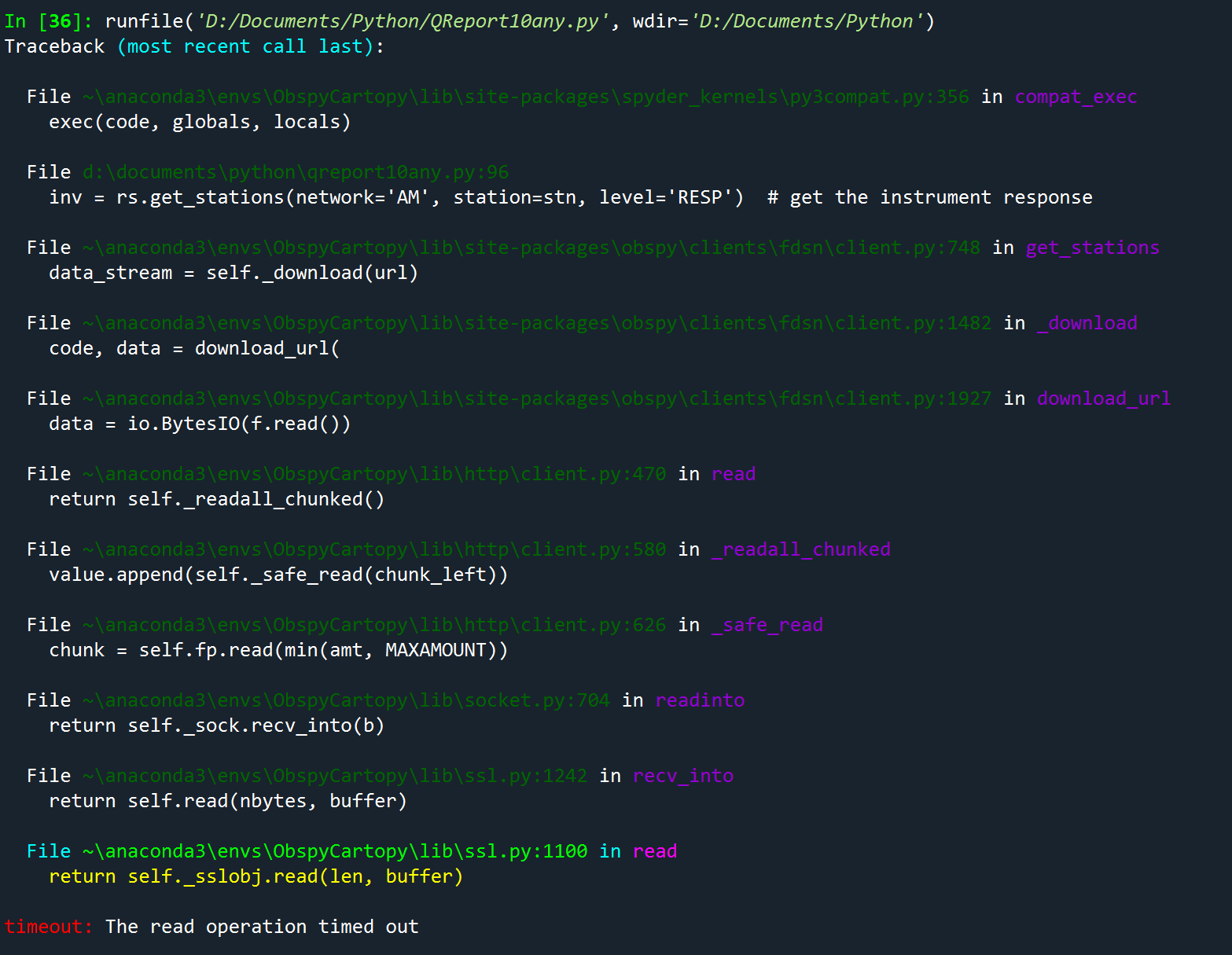
inv = rs.get_stations(network='AM', station=stn, level='RESP') # get the instrument response
sta = inv[0][0] #station metadata
latS = sta.latitude #station latitude
lonS = sta.longitude #station longitude
eleS = sta.elevation #station elevation
#enter event data
eventTime = UTCDateTime(2023, 5, 5, 5, 42, 4) # (YYYY, m, d, H, M, S) **** Enter data****
latE = 37.5 # quake latitude + N -S **** Enter data****
lonE = 137.3 # quake longitude + E - W **** Enter data****
depth = 9 # quake depth, km **** Enter data****
mag = 6.2 # quake magnitude **** Enter data****
eventID = 'rs2023iubjyd' # ID for the event **** Enter data****
locE = "Near West Coast of Honshu, Japan" # location name **** Enter data****
#Setup the data plot
delay = 200 # delay the start of the plot from the event **** Enter data****
duration = 900 # duration of plots **** Enter data****
notes1 = "" #add notes to the diagram. max one \n per note.
#notes1 = "Likely local noise at +596s, +608s. Refer to Spectrogram."
notes2 = ""
notes3 = ""
sandb = True #True if Raspberry Shake and Boom
if sandb:
sab = 'Raspberry Shake and Boom'
else:
sab = 'Raspberry Shake'
#set up the map
sat_height = 100000000.0 # adjust satellite height for desire view on map
lat_correction = 0 # correction in latutude for large distances
#set up the traces and ray paths
clear1tick = False #default is false. Set to True if first secondary axis ticks time overwrites the yaxis scale multiplier
plot_envelopes = False #plot envelopes on traces
allphases = True #true if all phases to be plotted, otherwise only those in the plotted time window are plotted **** Enter data****
save_plot = False #Set to True when plot is readyto be saved
start = eventTime + delay # calculate the plot start time from the event and delay
end = start + duration # calculate the end time from the start and duration
#set background noise sample times (choose a section of minimum velocity amplitude to represent background noise)
bnst = 900 # enter time of start of background noise sample (default = 0) **** Enter data****
bne = 600 # enter time of end of background noise sample (default = 600) **** Enter data****
bnstart = eventTime - bnst
bnend = eventTime + bne
# bandpass filter - select to suit system noise and range of quake
#filt = [0.1, 0.1, 0.8, 0.9]
#filt = [0.3, 0.3, 0.8, 0.9]
#filt = [0.5, 0.5, 2, 2.1]
filt = [0.7, 0.7, 2, 2.1] #distant quake
#filt = [0.7, 0.7, 3, 3.1]
#filt = [0.7, 0.7, 4, 4.1]
#filt = [0.7, 0.7, 6, 6.1]
#filt = [0.7, 0.7, 8, 8.1]
#filt = [1, 1, 10, 10.1]
#filt = [1, 1, 20, 20.1]
#filt = [3, 3, 20, 20.1] #use for local quakes
# set the FDSN server location and channel names
ch = 'EHZ' # ENx = accelerometer channels; EHx or SHZ = geophone channels
# get waveform and copy it for independent removal of instrument response
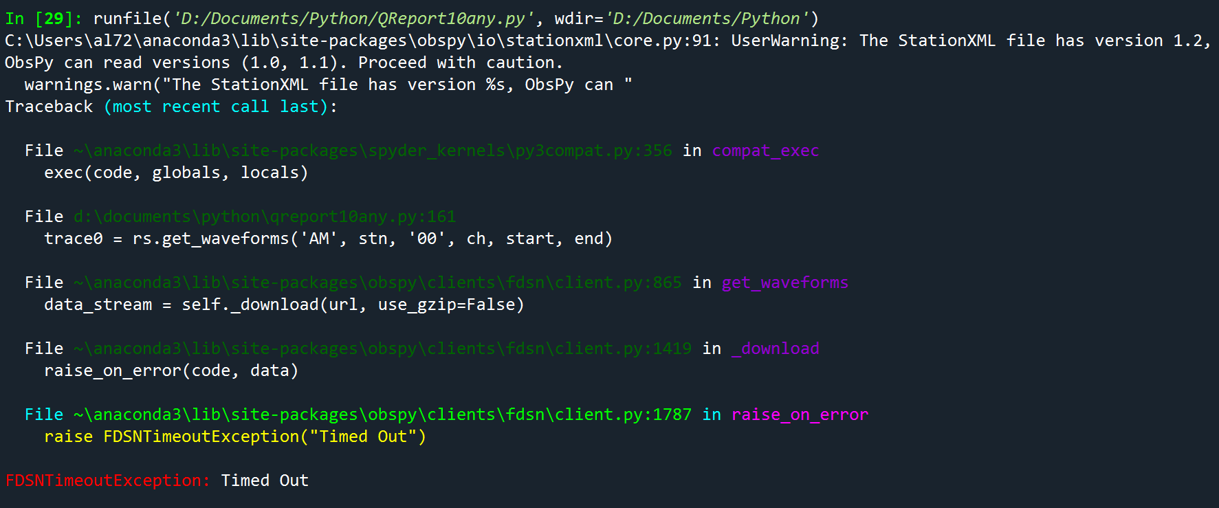
trace0 = rs.get_waveforms('AM', stn, '00', ch, start, end)
trace0.merge(method=0, fill_value='latest') #fill in any gaps in the data to prevent a crash
trace0.detrend(type='demean') #demean the data
trace1 = trace0.copy()
trace2 = trace0.copy()
rawtrace = trace0.copy() #save a raw copy of the trace for the spectrogram
#get waveform for background noise and copy it for independent removal of instrument response
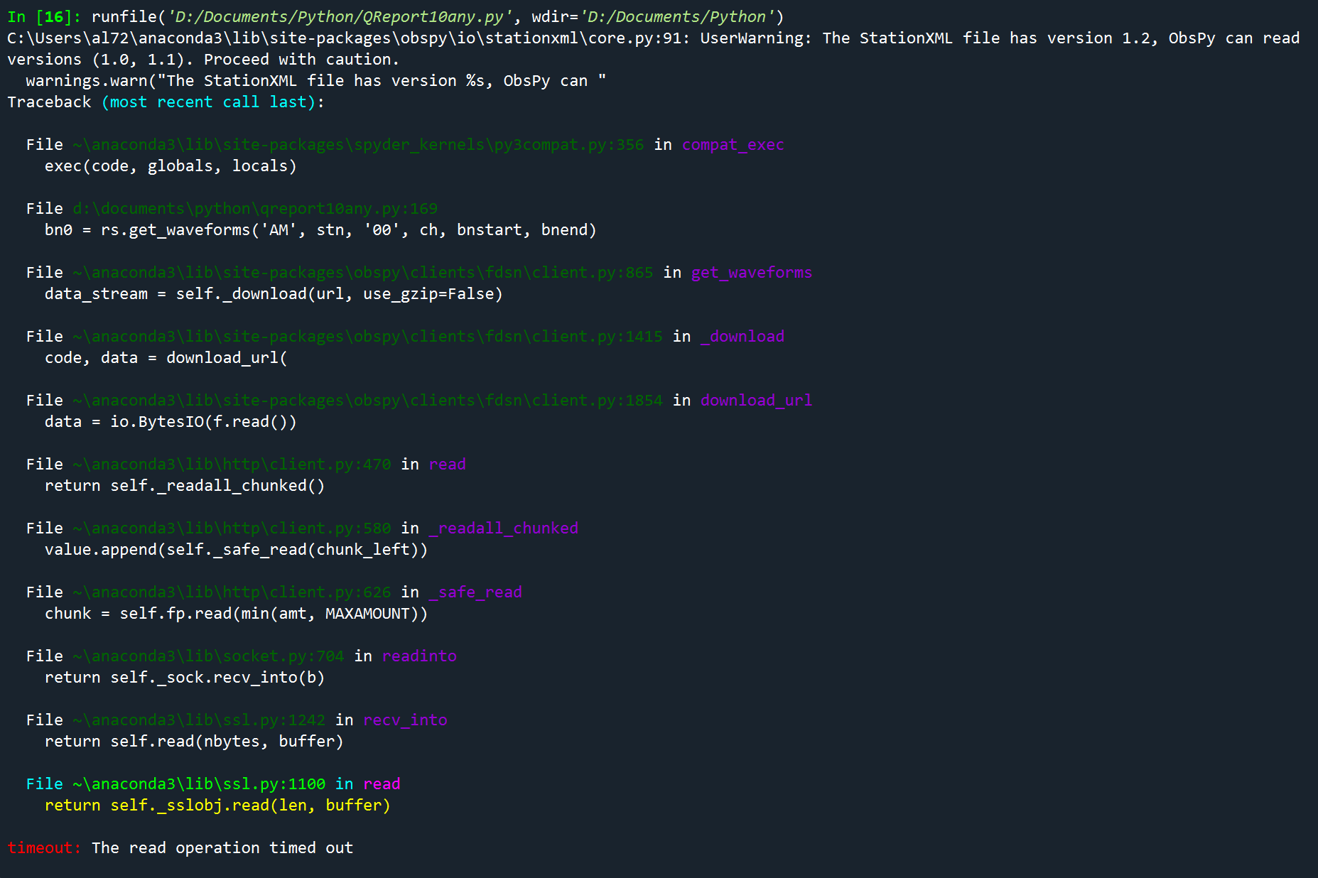
bn0 = rs.get_waveforms('AM', stn, '00', ch, bnstart, bnend)
bn0.merge(method=0, fill_value='latest') #fill in any gaps in the data to prevent a crash
bn0.detrend(type='demean') #demean the data
bn1 = bn0.copy() #copy for velocity
bn2 = bn0.copy() #copy for acceleration
# calculate great circle angle of separation
# convert angles to radians
latSrad = math.radians(latS)
lonSrad = math.radians(lonS)
latErad = math.radians(latE)
lonErad = math.radians(lonE)
if lonSrad > lonErad:
lon_diff = lonSrad - lonErad
else:
lon_diff = lonErad - lonSrad
great_angle_rad = math.acos(math.sin(latErad)*math.sin(latSrad)+math.cos(latErad)*math.cos(latSrad)*math.cos(lon_diff))
great_angle_deg = math.degrees(great_angle_rad) #great circle angle between quake and station
distance = great_angle_rad*12742/2 #calculate distance between quake and station in km
#Calculate the Phase Arrivals
model = TauPyModel(model='iasp91')
arrs = model.get_travel_times(depth, great_angle_deg)
print(arrs) # print the arrivals for reference when setting delay and duration
no_arrs = len(arrs) # the number of arrivals
#calculate Rayleigh Wave arrival Time
rayt = distance/2.96
print("Rayleigh Arrival Time: ", rayt)
# Calculate infrasound travel time for Boom signal
infraSL = distance/0.3062 #306.2m/s for -40°C
infraS0 = distance/0.331 #331m/s for 0°C
infraSE = distance/0.3547 #354.7m/s for +40°C
#Calculate Earthquake Total Energy
qenergy = 10**(1.5*mag+4.8)
# Create output traces
outdisp = trace0.remove_response(inventory=inv,pre_filt=filt,output='DISP',water_level=60, plot=False) # convert to Disp
outvel = trace1.remove_response(inventory=inv,pre_filt=filt,output='VEL',water_level=60, plot=False) # convert to Vel
outacc = trace2.remove_response(inventory=inv,pre_filt=filt,output='ACC',water_level=60, plot=False) # convert to Acc
#Calculate maximums
disp_max = outdisp[0].max()
vel_max = outvel[0].max()
acc_max = outacc[0].max()
se_max = vel_max*vel_max/2
#Create background noise traces
bndisp = bn0.remove_response(inventory=inv,pre_filt=filt,output='DISP',water_level=60, plot=False) # convert to Disp
bnvel = bn1.remove_response(inventory=inv,pre_filt=filt,output='VEL',water_level=60, plot=False) # convert to Vel
bnacc = bn2.remove_response(inventory=inv,pre_filt=filt,output='ACC',water_level=60, plot=False) # convert to Acc
# Calculate background noise limits using standard deviation
bnsamp = 15 #sample size in seconds
bns = int((bnend - bnstart)/bnsamp) #calculate the number of samples in the background noise traces
bnd = divTrace(bndisp[0],bns) #divide the displacement background noise trace into equal traces
bnv = divTrace(bnvel[0],bns) #divide the velocity background noise trace into equal traces
bna = divTrace(bnacc[0],bns) #divide the acceleration background noise trace into equal traces
for j in range (0, bns): #find the sample interval with the minimum background noise amplitude
if j == 0:
bndispstd = abs(bnd[j].std())
bnvelstd = abs(bnv[j].std())
bnaccstd = abs(bna[j].std())
elif abs(bnd[j].std()) < bndispstd:
bndispmax = abs(bnd[0].max())
elif abs(bnv[j].std()) < bnvelstd:
bnvelstd = abs(bnv[j].std())
elif abs(bna[j].max()) < bnaccstd:
bnaccstd = abs(bna[j].std())
bnsestd = bnvelstd*bnvelstd/2 #calculate the max background noise level for the specific energy
# Create Signal Envelopes
disp_env = filter.envelope(outdisp[0].data) #create displacement envelope
vel_env = filter.envelope(outvel[0].data) #create velocity envelope
acc_env = filter.envelope(outacc[0].data) #create acceleration envelope
se_env=vel_env*vel_env/2 #create specific energy envelope from velocity envelope!
#set up map plot
latC = (latE+latS)/2 #latitude 1/2 way between station and event/earthquake - may need adjusting!
lonC = (lonE+lonS)/2 #longitude 1/2 way between station and event/earthquake - may need adjusting!
if abs(lonE-lonS) > 180:
lonC = lonC + 180
projection=ccrs.NearsidePerspective(
central_latitude=latC + lat_correction,
central_longitude=lonC,
satellite_height=sat_height) #adjust satellite height to best display station and event/earthquake
# set up plot
fig = plt.figure(figsize=(20,14), dpi=150) # set to page size in inches
ax1 = fig.add_subplot(6,2,1) # displacement waveform
ax2 = fig.add_subplot(6,2,3) # velocity Waveform
ax3 = fig.add_subplot(6,2,5) # acceleration waveform
ax6 = fig.add_subplot(6,2,7) # specific energy waveform
ax4 = fig.add_subplot(6,2,9) # velocity spectrogram
ax5 = fig.add_subplot(6,2,11) # velocity PSD
ax7 = fig.add_subplot(6,2,(2,6), polar=True) # TAUp plot
ax8 = fig.add_subplot(6,2,(8,12), projection=projection)
fig.suptitle("M"+str(mag)+" Earthquake - "+locE+" - "+eventTime.strftime(' %d/%m/%Y %H:%M:%S UTC'), weight='black', color='b', size='x-large') #Title of the figure
fig.text(0.05, 0.95, "Filter: "+str(filt[1])+" to "+str(filt[2])+"Hz") # Filter details
fig.text(0.51, 0.055, 'Separation = '+str(round(great_angle_deg,3))+u"\N{DEGREE SIGN}"+' or '+str(int(distance))+'km.') #distance between quake and station
fig.text(0.51, 0.04, 'Latitude: '+str(latE)+u"\N{DEGREE SIGN}"+' Longitude: '+str(lonE)+u"\N{DEGREE SIGN}"+' Depth: '+str(depth)+'km.') #quake lat, lon and depth
fig.text(0.51, 0.07, 'Quake Energy: '+f"{qenergy:0.1E}"+'J.') #Earthquake energy
fig.text(0.7, 0.95, 'Event ID: '+eventID)
fig.text(0.95, 0.95, 'Station: AM.'+stn+'.00.'+ch, ha='right',size='large')
fig.text(0.95, 0.935, sab, color='r', ha='right')
fig.text(0.95, 0.92, '#ShakeNet', ha='right')
fig.text(0.95, 0.905, '@raspishake', ha='right')
fig.text(0.95, 0.89, '@AlanSheehan18', ha='right')
fig.text(0.95, 0.875, '@matplotlib', ha='right')
fig.text(0.98, 0.86, '#Python', ha='right')
fig.text(0.98, 0.845, '#CitizenScience', ha='right')
fig.text(0.98, 0.83, '#Obspy', ha='right')
fig.text(0.98, 0.815, '#Cartopy', ha='right')
# plot logos
pics = "D:/Pictures/Raspberry Shake and Boom/"
rsl = plt.imread(pics+"RS logo.png")
twl = plt.imread(pics+"twitter logo.png")
newaxr = fig.add_axes([0.935, 0.915, 0.05, 0.05], anchor='NE', zorder=-1)
newaxr.imshow(rsl)
newaxr.axis('off')
newaxt = fig.add_axes([0.943, 0.878, 0.04, 0.04], anchor='NE', zorder=-1)
newaxt.imshow(twl)
newaxt.axis('off')
#perspective map viewing height
fig.text(0.885, 0.05, 'Satellite Viewing Height = '+str(int(sat_height/1000))+' km.', rotation=90)
#print notes
fig.text(0.90, 0.03, 'NOTES: '+notes1, rotation=90)
fig.text(0.917, 0.03, notes2, rotation=90)
fig.text(0.934, 0.03, notes3, rotation=90)
#end trace notes and maxima
fig.text(0.48, 0.715, 'Energy is', size='x-small',rotation=90, va='center')
fig.text(0.485, 0.715, 'proportional to V²', size='x-small',rotation=90, va='center')
fig.text(0.48, 0.87, 'Displacement biases', size='x-small',rotation=90, va='center')
fig.text(0.485, 0.87, 'low frequencies', size='x-small',rotation=90, va='center')
fig.text(0.48, 0.56, 'Acceleration biases', size='x-small',rotation=90, va='center')
fig.text(0.485, 0.56, 'high frequencies', size='x-small',rotation=90, va='center')
fig.text(0.48, 0.41, 'E/m = v²/2', size='x-small',rotation=90, va='center')
fig.text(0.485, 0.41, 'For weak arrivals', size='x-small',rotation=90, va='center')
fig.text(0.49, 0.87, 'Max D = '+f"{disp_max:.3E}"+' m', size='small',rotation=90, va='center',color='b')
fig.text(0.49, 0.715, 'Max V = '+f"{vel_max:.3E}"+' m/s', size='small',rotation=90, va='center',color='g')
fig.text(0.49, 0.56, 'Max A = '+f"{acc_max:.3E}"+' m/s²', size='small',rotation=90, va='center',color='r')
fig.text(0.49, 0.41, 'Max SE = '+f"{se_max:.3E}"+' J/kg', size='small',rotation=90, va='center',color='g')
fig.text(0.48, 0.253, 'Unfiltered Spectrogram', size='x-small', rotation=90, va='center')
# print signal to noise ratios
fig.text(0.495, 0.87, 'S/N = '+f"{abs(disp_max/(3*bndispstd)):.3}", size='x-small', rotation=90, va='center', color='b')
fig.text(0.495, 0.715, 'S/N = '+f"{abs(vel_max/(3*bnvelstd)):.3}", size='x-small', rotation=90, va='center', color='g')
fig.text(0.495, 0.56, 'S/N = '+f"{abs(acc_max/(3*bnaccstd)):.3}", size='x-small', rotation=90, va='center', color='r')
fig.text(0.495, 0.41, 'S/N = '+f"{abs(se_max/(3*bnsestd)):.3}", size='x-small', rotation=90, va='center', color='g')
# print background noise data
fig.text(0.51, 0.3, 'Background Noise:', size='small')
fig.text(0.51, 0.29, 'Displacement:', color='b', size='small')
fig.text(0.51, 0.28, 'SD = '+f"{bndispstd:.3E}"+' m', color='b', size='small')
fig.text(0.51, 0.27, '3SD = '+f"{(3*bndispstd):.3E}"+' m', color='b', size='small')
fig.text(0.51, 0.26, 'Velocity:', color='g', size='small')
fig.text(0.51, 0.25, 'SD = '+f"{bnvelstd:.3E}"+' m/s', color='g', size='small')
fig.text(0.51, 0.24, '3SD = '+f"{(3*bnvelstd):.3E}"+' m/s', color='g', size='small')
fig.text(0.51, 0.23, 'Acceleration:', color='r', size='small')
fig.text(0.51, 0.22, 'SD = '+f"{bnaccstd:.3E}"+' m/s²', color='r', size='small')
fig.text(0.51, 0.21, '3SD = '+f"{(3*bnaccstd):.3E}"+' m/s²', color='r', size='small')
fig.text(0.51, 0.20, 'Specific Energy:', color='g', size='small')
fig.text(0.51, 0.19, 'SD = '+f"{bnsestd:.3E}"+' J/kg', color='g', size='small')
fig.text(0.51, 0.18, '3SD = '+f"{(3*bnsestd):.3E}"+' J/kg', color='g', size='small')
fig.text(0.51, 0.17, 'BN parameters:', size='small')
fig.text(0.51, 0.16, 'Minimum SD over:', size='small')
fig.text(0.51, 0.15, 'Start: Event time - '+str(bnst)+' s.',size='small')
fig.text(0.51, 0.14, 'End: Event time + '+str(bne)+' s.',size='small')
fig.text(0.51, 0.13, 'BN Sample size = '+str(bnsamp)+' s.',size='small')
#plot traces
ax1.plot(trace0[0].times(reftime=eventTime), outdisp[0].data, lw=1, color='b') # displacement waveform
fmtax(ax1, 0, False) #axis, limit, no negatives
ax2.plot(trace0[0].times(reftime=eventTime), outvel[0].data, lw=1, color='g') # velocity Waveform
fmtax(ax2, 0, False) #axis, limit, no negatives
ax3.plot(trace0[0].times(reftime=eventTime), outacc[0].data, lw=1, color='r') # acceleration waveform
fmtax(ax3, 0, False) #axis, limit, no negatives
ax4.specgram(x=rawtrace[0], NFFT=100, noverlap=0, Fs=100, cmap='viridis') # velocity spectrogram
#ax4.specgram(trace0[0].times(reftime=eventTime), rawtrace[0].data, NFFT=100, noverlap=0, Fs=100, cmap='viridis') # velocity spectrogram
ax4.xaxis.set_minor_locator(AutoMinorLocator(10))
ax4.set_yscale('log') # set logarithmic y scale
ax4.set_ylim(0.5,50) #limits for log scale
#plot filter limits on spectrogram
ax4.axhline(y=filt[1], lw=1, color='r', linestyle='dotted')
ax4.axhline(y=filt[2], lw=1, color='r', linestyle='dotted')
#ax5.psd(x=rawtrace[0], NFFT=512, noverlap=0, Fs=100, color='k', lw=1) # velocity PSD raw data
ax5.psd(x=trace0[0], NFFT=512, noverlap=0, Fs=100, color='b', lw=1) # displacement PSD filtered
ax5.psd(x=trace1[0], NFFT=512, noverlap=0, Fs=100, color='g', lw=1) # velocity PSD filtered
ax5.psd(x=trace2[0], NFFT=512, noverlap=0, Fs=100, color='r', lw=1) # acceleration PSD filtered
ax5.set_xscale('log') #use logarithmic scale on PSD
#plot filter limits on PSD
ax5.axvline(x=filt[1], linewidth=1, linestyle='dotted', color='r')
ax5.axvline(x=filt[2], linewidth=1, linestyle='dotted', color='r')
ax6.plot(trace0[0].times(reftime=eventTime), outvel[0].data*outvel[0].data/2, lw=1, color='g', linestyle=':') #specific kinetic energy Waveform
fmtax(ax6, 0, True) #axis, limit, no negatives
#plot background noise limits
plot_noiselims(ax1, bndispstd, -bndispstd) #displacement noise limits
plot_noiselims(ax2, bnvelstd, -bnvelstd) #velocity noise limits
plot_noiselims(ax3, bnaccstd, -bnaccstd) #acceleration noise limits
plot_se_noiselims(ax6, bnsestd) #specific kinetic energy noise limits
# plot Signal envelopes
if plot_envelopes:
ax1.plot(trace0[0].times(reftime=eventTime), disp_env, 'b:') #displacement envelope
ax2.plot(trace0[0].times(reftime=eventTime), vel_env, 'g:') #velocity envelope
ax3.plot(trace0[0].times(reftime=eventTime), acc_env, 'r:') #acceleration envelope
#envelope for specific kinetic plot IS the specific energy graph.
#Energy is a scalar, so in vibrations alternates between kinetic and potential energy states.
ax6.plot(trace0[0].times(reftime=eventTime), se_env, 'g') #specific energy envelope
#plot secondary axes - set time interval (dt) based on the duration to avoid crowding
if duration <= 90:
dt=10 #10 seconds
elif duration <= 180:
dt=20 #20 seconds
elif duration <= 270:
dt=30 #30 seconds
elif duration <= 540:
dt=60 #1 minute
elif duration <= 1080:
dt=120 #2 minutes
elif duration <= 2160:
dt=240 #4 minutes
else:
dt=300 #5 minutes
tbase = start - start.second +(int(start.second/dt)+1)*dt #find the first time tick
tlabels = [] #initialise a blank array of time labels
tticks = [] #initialise a blank array of time ticks
sticks = [] #initialise a blank array for spectrogram ticks
nticks = int(duration/dt) #calculate the number of ticks
for k in range (0, nticks):
if k==0 and clear1tick:
tlabels.append('')
elif dt >= 60: #build the array of time labels - include UTC to eliminate the axis label
tlabels.append((tbase+k*dt).strftime('%H:%M UTC')) #drop the seconds if not required for readability
else:
tlabels.append((tbase+k*dt).strftime('%H:%M:%SUTC')) #include seconds where required
tticks.append(uTC2time(tbase+k*dt)) #build the array of time ticks
sticks.append(uTC2time(tbase+k*dt)-delay) #build the array of time ticks for the spectrogram
print(tlabels)
print(tticks)
secax_x1 = ax1.secondary_xaxis('top') #Displacement secondary axis
sax(secax_x1, tticks)
secax_x2 = ax2.secondary_xaxis('top') #Velocity secondary axis
sax(secax_x2, tticks)
secax_x3 = ax3.secondary_xaxis('top') #acceleration secondary axis
sax(secax_x3, tticks)
secax_x4 = ax4.secondary_xaxis('top') #spectrogram secondary axis
sax(secax_x4, sticks)
secax_x6 = ax6.secondary_xaxis('top') #Specific Energy secondary axis
sax(secax_x6, tticks)
secax_x5 = ax5.secondary_xaxis('top', functions=(one_over, inverse)) #PSD secondary axis
secax_x5.set_xlabel('Period, s', size='small', labelpad=-3)
#add grid to graphs
ax4.grid(color='dimgray', ls = '-.', lw = 0.33)
grid(ax5)
#plot map
ax8.coastlines(resolution='110m')
ax8.stock_img()
# Create a feature for States/Admin 1 regions at 1:50m from Natural Earth to display state borders
states_provinces = cfeature.NaturalEarthFeature(
category='cultural',
name='admin_1_states_provinces_lines',
scale='50m',
facecolor='none')
ax8.add_feature(states_provinces, edgecolor='gray')
ax8.gridlines()
#plot station position on map
ax8.plot(lonS, latS,
color='red', marker='v', markersize=12, markeredgecolor='black',
transform=ccrs.Geodetic(),
)
#plot event/earthquake position on map
ax8.plot(lonE, latE,
color='yellow', marker='*', markersize=20, markeredgecolor='black',
transform=ccrs.Geodetic(),
)
#plot dashed great circle line from event/earthquake to station
ax8.plot([lonS, lonE], [latS, latE],
color='blue', linewidth=2, linestyle='--',
transform=ccrs.Geodetic(),
)
# build array of arrival data
y2 = 0.93 #start near middle of page but maximise list space
dy = 0.01 # linespacing
fig.text(0.505, y2, 'Phase',size='xx-small') #print headings
fig.text(0.53, y2, 'Time',size='xx-small')
fig.text(0.555, y2, 'UTC',size='xx-small')
fig.text(0.575, y2, 'Vertical Component', size='xx-small')
pphases=[] #create an array of phases to plot
pfile='' #create phase names for filename
alf=1.0 #set default transparency
for i in range (0, no_arrs): #print data array
y2 -= dy
if arrs[i].time >= delay and arrs[i].time < (delay+duration): #list entries in the plots are black
alf=1.0
else: #list entries not in plots are greyed out
alf=0.5
fig.text(0.505, y2, arrs[i].name, size='xx-small', alpha=alf) #print phase name
fig.text(0.53, y2, str(round(arrs[i].time,3))+'s', size='xx-small', alpha=alf) #print arrival time
arrtime = eventTime + arrs[i].time
fig.text(0.555, y2, arrtime.strftime('%H:%M:%S'), size='xx-small', alpha=alf)
if allphases or (arrs[i].time >= delay and arrs[i].time < (delay+duration)): #build the array of phases
pphases.append(arrs[i].name)
pfile += ' '+arrs[i].name
if arrs[i].name.endswith('P') or arrs[i].name.endswith('p') or arrs[i].name.endswith('Pdiff') or arrs[i].name.endswith('Pn'): #calculate and print the vertical component of the signal
fig.text(0.575, y2, str(round(100*math.cos(math.radians(arrs[i].incident_angle)),1))+'%', alpha = alf, size='xx-small')
elif arrs[i].name.endswith('S') or arrs[i].name.endswith('s') or arrs[i].name.endswith('Sn') or arrs[i].name.endswith('Sdiff'):
fig.text(0.575, y2, str(round(100*math.sin(math.radians(arrs[i].incident_angle)),1))+'%', alpha = alf, size='xx-small')
y2 -= 2*dy
fig.text(0.505, y2, str(no_arrs)+' arrivals total.', size='xx-small') #print number of arrivals
print(pphases)
if allphases or (rayt >= delay and rayt <= (delay+duration)):
y2 -= 2*dy
fig.text(0.505, y2, 'Rayleigh', size='xx-small')
y2 -= dy
fig.text(0.505, y2, 'Surface Wave: '+str(round(rayt,1))+'s:', size='xx-small')
arrtime = eventTime + rayt
fig.text(0.555, y2, arrtime.strftime('%H:%M:%S UTC'), size='xx-small')
#print infrasound arrival window
if allphases:
y2 -= 2*dy
fig.text(0.505, y2, 'Infrasound Window', size='xx-small')
y2 -= dy
fig.text(0.505, y2, 'Start: '+str(round(infraSE,1))+'s:', size='xx-small')
arrtime = eventTime + infraSE
fig.text(0.555, y2, arrtime.strftime('%H:%M:%S UTC'), size='xx-small')
y2 -= dy
fig.text(0.505, y2, 'Median: '+str(round(infraS0,1))+'s:', size='xx-small')
arrtime = eventTime + infraS0
fig.text(0.555, y2, arrtime.strftime('%H:%M:%S UTC'), size='xx-small')
y2 -= dy
fig.text(0.505, y2, 'End: '+str(round(infraSL,1))+'s:', size='xx-small')
arrtime = eventTime + infraSL
fig.text(0.555, y2, arrtime.strftime('%H:%M:%S UTC'), size='xx-small')
# print phase key
y2 = 0.62 # line spacing
fig.text(0.98, y2, 'Phase Key', size='small', ha='right') #print heading
pkey = ['P: compression wave', 'p: strictly upward compression wave', 'S: shear wave', 's: strictly upward shear wave', 'K: compression wave in outer core', 'I: compression wave in inner core', 'c: reflection off outer core', 'diff: diffracted wave along core mantle boundary', 'i: reflection off inner core', 'n: wave follows the Moho (crust/mantle boundary)']
for i in range (0, 10):
y2 -=dy
fig.text(0.98, y2, pkey[i], size='x-small', ha='right') #print the phase key
#plot phase arrivals
plot_arrivals(ax1,0) #plot arrivals on displacement plot
plot_arrivals(ax2,0) #plot arrivals on velocity plot
plot_arrivals(ax3,0) #plot arrivals on acceleration plot
plot_arrivals(ax4,delay) #plot arrivals on spectrogram plot
plot_arrivals(ax6,0) #plot arrivals on energy plot
# set up some plot details
ax1.set_ylabel("Vertical Displacement, m", size='small')
ax2.set_ylabel("Vertical Velocity, m/s", size ='small')
ax3.set_ylabel("Vertical Acceleration, m/s²", size='small')
ax4.set_ylabel("Velocity Frequency, Hz", size='small')
ax4.set_xlabel('Seconds after Start of Trace, s', size='small', labelpad=0)
ax5.set_ylabel("PSD, dB",size='small')
ax5.set_xlabel('Frequency, Hz', size='small', labelpad=0)
ax6.set_ylabel('Specific Energy, J/kg', size='small')
# get the limits of the y axis so text can be consistently placed
ax4b, ax4t = ax4.get_ylim()
ax4.text(2, ax4t*0.6, 'Plot Start Time: '+start.strftime(' %d/%m/%Y %H:%M:%S.%f UTC (')+str(delay)+' seconds after event).', size='small') # explain difference in x time scale
#adjust subplots for readability
plt.subplots_adjust(hspace=0.5, wspace=0.1, left=0.05, right=0.95, bottom=0.05, top=0.92)
#plot the ray paths
arrivals = model.get_ray_paths(depth, great_angle_deg, phase_list=pphases) #calculate the ray paths
ax7 = arrivals.plot_rays(plot_type='spherical', ax=ax7, fig=fig, phase_list=pphases, show=False, legend=True) #plot the ray paths
if allphases:
fig.text(0.91, 0.71, 'Show All Phases', size='small')
else:
fig.text(0.91, 0.71, 'Show Phases\nVisible in Traces', size='small')
if great_angle_deg > 103 and great_angle_deg < 143:
ax7.text(great_angle_rad,6000, 'Station in P and\nS wave shadow', size='x-small', rotation=180-great_angle_deg, ha='center', va='center')
elif great_angle_deg >143:
ax7.text(great_angle_rad,6000, 'Station in S\nwave shadow', size='x-small', rotation=180-great_angle_deg, ha='center', va='center')
#label Station
ax7.text(great_angle_rad,7000, stn, ha='center', va='center', alpha=.7, size='small', rotation= -great_angle_deg)
# add boundary depths
ax7.text(math.radians(315),5550, '660km', ha='center', va='center', alpha=.7, size='small', rotation=45)
ax7.text(math.radians(315),3300, '2890km', ha='center', va='center', alpha=.7, size='small', rotation=45)
ax7.text(math.radians(315),1010, '5150km', ha='center', va='center', alpha=.7, size='small', rotation=45)
# Annotate regions
ax7.text(0, 0, 'Solid\ninner\ncore',
horizontalalignment='center', verticalalignment='center',
bbox=dict(facecolor='white', edgecolor='none', alpha=0.7))
ocr = (model.model.radius_of_planet -
(model.model.s_mod.v_mod.iocb_depth +
model.model.s_mod.v_mod.cmb_depth) / 2)
ax7.text(math.radians(180), ocr, 'Fluid outer core',
horizontalalignment='center',
bbox=dict(facecolor='white', edgecolor='none', alpha=0.7))
mr = model.model.radius_of_planet - model.model.s_mod.v_mod.cmb_depth / 2
ax7.text(math.radians(180), mr, 'Solid mantle',
horizontalalignment='center',
bbox=dict(facecolor='white', edgecolor='none', alpha=0.7))
#create phase identifier for filename
if allphases:
pfile = ' All'
#print filename on bottom left corner of diagram
filename = pics+'M'+str(mag)+'Quake '+locE+eventID+eventTime.strftime('%Y%m%d %H%M%S UTC'+stn+pfile+'.png')
fig.text(0.02, 0.01,filename, size='x-small')
# save the final figure
if save_plot:
plt.savefig(filename)
# show the final figure
plt.show()
The most likely thing I can think of in my code might be the sta=inv[0][0] in line 97. I used to enter the stattion latitude, longitude and elevation manually for my station but added that code to be able to use the program on any station. Pretty sure I don’t remember any timeouts before I made that mod…
Al.
Hello sheeny,
Thank you for the entire code. I’ve tested it in my ObsPy environment, but, except for a missing logo warning (that I was able to bypass by commenting out that line), I didn’t manage to replicate the timeouts error you are seeing.
Are them still happening? And, as a standard question, if you remove the sta=inv[0][0] on line 97, do they disappear, or are still there?
G’Day Stormchaser,
I don’t think I’ve had one instance of a timeout since reporting it, but I haven’t had a lot of quakes to process either. I’ll do some testing today and just repeatedly run the program and see if I can get a timeout to occur.
The faults report as being from the get_station or get_waveform commands, so I don’t know how they can be the result of the sta=inv[0][0]… that was simply the last change the program that I’d made before they started occurring. If I find any timeouts with the existing code, I’ll run an older version and see if I can get it to do it.
Al.
G’Day again,
I’ve just run my report 30 times and no timeouts.
I wonder if it may be traffic related? I don’t know if that’s possible, but the couple of days I had the issue I had detected quite a few largish earthquakes, so I was processing more than average. If a lot of other shakers were doing the same, maybe it was traffic on the server?
Al.
Good evening sheeny,
At this point, as the issue has not appeared again for you, and I have the same behaviour, we can probably correlate it to either traffic load and/or some kind of internet-related problem along your lines that was then corrected later.
In any case, happy that everything now works properly! Your feedback is always valuable.
After the timeouts this morning, I ran an old version of my report (without the sta=inv[0][0] command) and on the final time it also gave a timeout, so the timeouts are not related to the sta=inv[0][0] command.
Al.
Hello sheeny,
I’ve just finished checking on our servers and our FDSN service, but everything is running without issues as far as I can see, even during the night. It must be something else that is causing the problem you’re seeing now, even if I’m unsure on what it could be.
One thing I noticed is that you are using an older version of ObsPy (probably v1.3.0?) which is cause of the warning you see in lines 2-4 of your screenshots. Can you update it to the latest version and see if this yields any positive effect?
G’day Stormchaser,
Anaconda wasn’t letting me update obspy, so I’ve had to create a new environment for Obspy and Cartopy and so I’m finally on v1.4.0.
Time will tell if this makes a difference.
Thanks,
Al.
Hello sheeny,
I’ve rechecked our servers in the hours before your message (and a bit after, just to be sure), but no issue has been found. All systems were performing nominally at the time, so we didn’t have an outage that could have caused the read operation timeout as you have highlighted.
Have you noticed a pattern in the timeouts themselves? That is, if they happen at certain times of the day/week or if they happen when you request more data more frequently, or anything else that comes to mind? That could give us a clue on what to look for.
G’Day Stormchaser,
I am away from home this week, but prior to leaving I did some speed tests on my internet connection at home and found a great deal of variability. I think I might have some issues to sort out with my service provider, but that said, what I’m seeing on my internet connection would only explain slow downloads.
The inventory and waveform data I would not expect to be anywhere near as bandwidth hungry as live streaming video, yet it times out - which is a long time. It’s almost live the data request is lost before it gets to the FDSN server, and I don’t know if that’s possible.
Thanks for your help. It’s looking increasingly to me that the problem is my end, which is frustrating.
Thanks for your help,
Al.
Hello sheeny,
Thanks to you for the time and effort you are dedicating to this issue that you are experiencing. Regarding this,
It’s almost live the data request is lost before it gets to the FDSN server
It would be possible only if the connection is interrupted before the data request makes it through, which I also think it’s a difficult concatenation of events, especially if other devices in your house do not experience similar connection problems.
Please keep us updated on what you are able to find in the coming days, I think this thread could become a reference point for other users who are experiencing similar issues.
For future reference, the National Broadband Network (NBN) are doing capacity work in my area early next month. Hopefully that will help. My typical download speeds have been 18 to 25MB/s but occasionally I have found it as low as 8MB/s with gaps of zero!
It is worth noting though that at times when I have had timeouts subsequent speed test have been up in the 18 to 25MB/s range, so local speed is not the only problem. I haven’t tried to run a speed test to the server to test the whole network.
Al.