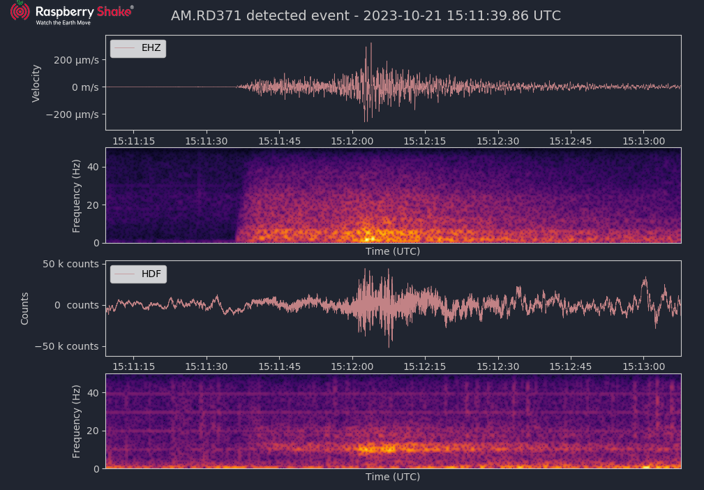
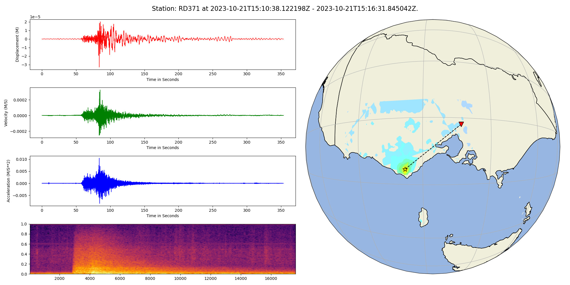
Last night while I was trying to sleep the alarm function I set up with rsudp went off and I thought it was someone who went near it but no! I barely felt the earthquake myself but I could tell something was happening and it kind of acted like an early warning which was cool
5 Likes
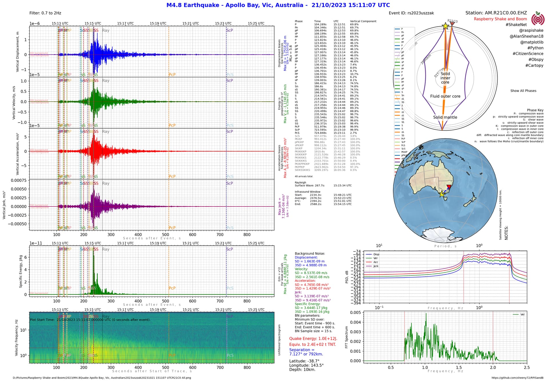
Cool plots, I’ve been working on my own the for the past day or so but no where near that quality yet ![]()
3 Likes
That’s cool, Matt. Nice and elegant.
It takes time. ;o) Being retired I have plenty of time to play with my reports and code, and it probably shows as I tend to cram a lot into my reports (just because I can ;o) ).
Al.
4 Likes
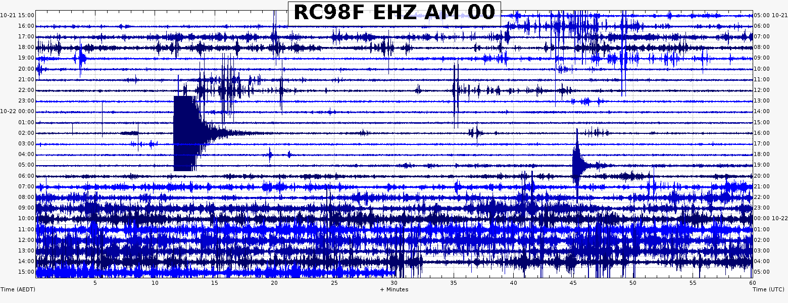
RC98F here - just North of Ballarat, Victoria.
It’s nice to see the neighbourhood activity, and the spiffy charts!
We slept right through it but family in Ballarat did feel it.
3 Likes
G’Day Graibeard!
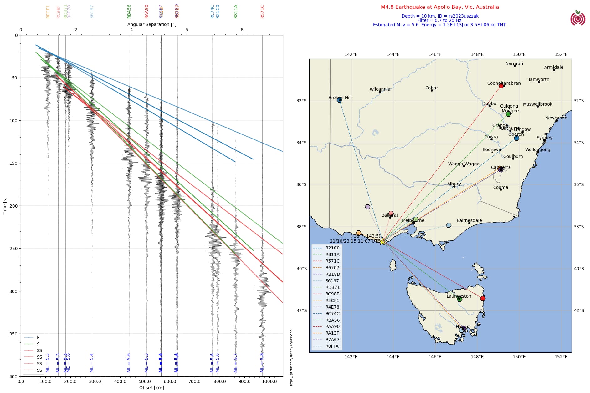
Welcome aboard. Here’s another plot with your station in it… ;o)
Another aftershock today:
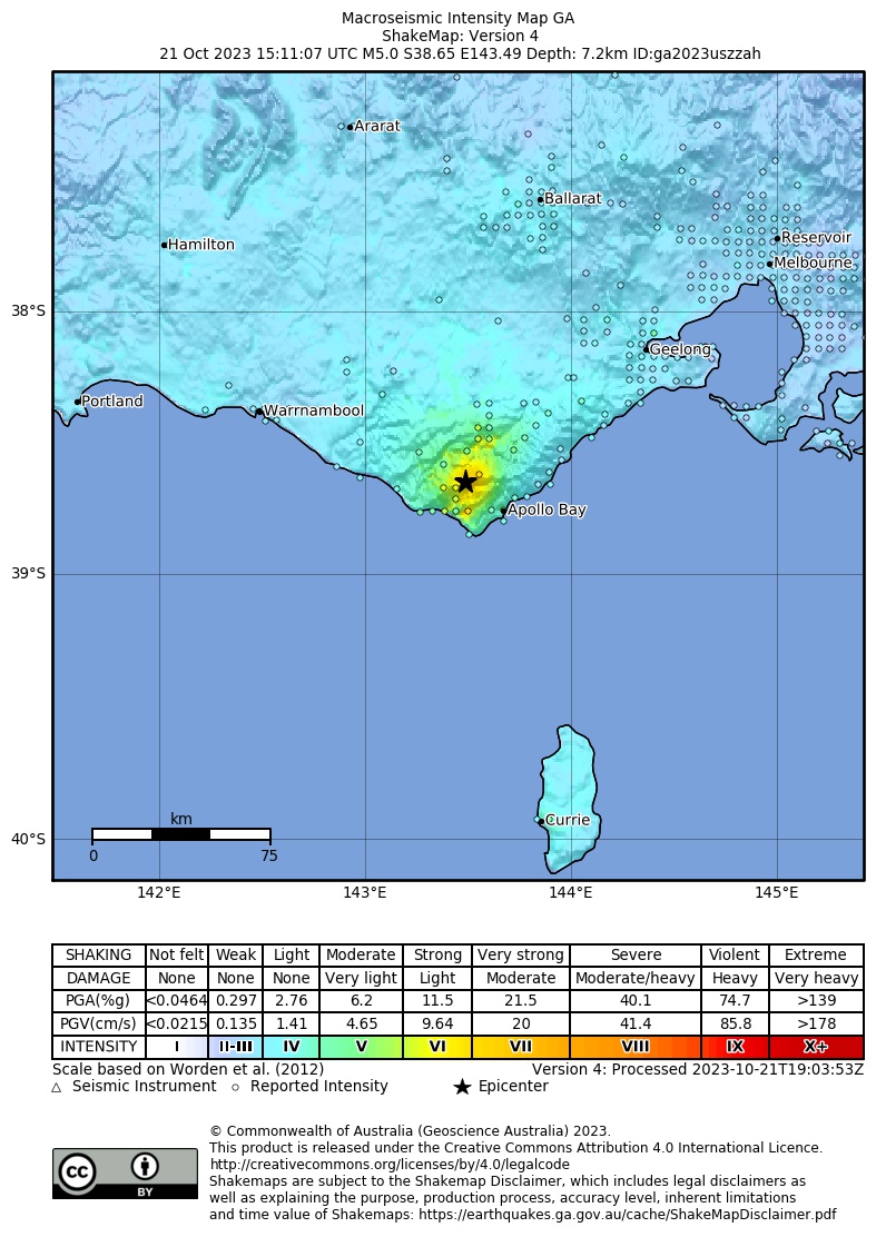
I see the “official” name for the location of the quake is the Otway Ranges (at least amongst Australian Seismologists). I usually plug the lat and long into Google maps and use the locality name it provides to add a more local feel to it. I was slack and didn’t do that on my previous report - I just thought it’s close enough to Apollo Bay. This time I used the Google Maps locality name.
Al.
4 Likes
Hey sheeny, I have a question about getting data for the record section.
How do you get the waveforms without getting Request would result in too much data. Denied by the datacenter. Split the request in smaller parts?
My current code for that is:
invs = rs.get_stations(network='AM', latitude=lat, longitude=lon, maxradius=2, level='RESP')
stns = invs[0].stations
channels = ['EHZ']

stream = Stream()
for stn in stns:
    print(stn)
    for ch in channels:
        trace = rs.get_waveforms('AM', stn, '00', ch, start, end)
        stream += trace
3 Likes
G’Day Matt.
Hmmm…
It looks like you are trying to get the get_stations command to find the stations within a radius of a lat long. I haven’t done that, but I think the problem may be that you haven’t got a starttime and endtime in the get_stations command. I think the get_station command gets a lot more than the just the station name, so try the starttime and endtime and see if that fixes the problem.
My approach was different. I manually compile the list of stations I want to use, and use that to drive the get_stations command in a loop to get the instrument responses and to build the stream.
FWIW I’m happy to share my code, even though it’s not the same approach, it might trigger something. Feel free to use as much as you want. ;o)
Al.
# -*- coding: utf-8 -*-
"""
Created on Sun May 21 12:22:53 2023
@author: al72
"""
from obspy.clients.fdsn import Client
from obspy.core import UTCDateTime, Stream
import matplotlib.pyplot as plt
from obspy.taup import TauPyModel
import cartopy.crs as ccrs
import cartopy.feature as cfeature
import numpy as np
from matplotlib.transforms import blended_transform_factory
from matplotlib.cm import get_cmap
from obspy.geodetics import gps2dist_azimuth, kilometers2degrees, degrees2kilometers
from matplotlib.ticker import AutoMinorLocator
rs = Client('https://data.raspberryshake.org/')
# Build a station list of local stations so unwanted stations can be commented out
# as required to save typing
def stationList(sl):
sl += ['R21C0'] #Oberon
sl += ['R811A'] #Mudgee
#sl += ['R9AF3'] #Gulgong
sl += ['R571C'] #Coonabarabran
#sl += ['R6D2A'] #Coonabarabran
#sl += ['RF35D'] #Narrabri
#sl += ['R7AF5'] #Muswellbrook
#sl += ['R26B1'] #Murrumbateman
#sl += ['R3756'] #Chatswood
#sl += ['R9475'] #Sydney
sl += ['R6707'] #Gungahlin
#sl += ['R69A2'] #Penrith
sl += ['RB18D'] #Canberra
#sl += ['R9A9D'] #Brisbane
#sl += ['RCF6A'] #Brisbane
sl += ['S6197'] #Heyfield
sl += ['RD371'] #Melbourne
sl += ['RC98F'] #Creswick
#sl += ['RA20F'] #Broken Hill
#sl += ['RC74C'] #Broken Hill
sl += ['RECF1'] #Koroit
sl += ['R4E78'] #Stawell
sl += ['RC74C'] #Broken Hill
#sl += ['RDD97'] #Melbourne
#sl += ['R9CDF'] #Dandenong
sl += ['RBA56'] #Launceston
sl += ['RAA90'] #Scamander
sl += ['RA13F'] #Hobart
sl += ['R7A67'] #Hobart
sl += ['R0FFA'] #Hobart
#print(sl)
return sl
# Build a stream of traces from each of the selected stations
def buildStream(strm):
n = len(slist) # n is the number of traces (stations) in the stream
tr1 = []
for i in range(0, n):
inv = rs.get_stations(network='AM', station=slist[i], level='RESP') # get the instrument response
#read each epoch to find the one that's active for the event
k=0
while True:
sta = inv[0][k] #station metadata
if sta.is_active(time=eventTime):
break
k += 1
latS = sta.latitude #active station latitude
lonS = sta.longitude #active station longitude
#eleS = sta.elevation #active station elevation is not required for this program
print(sta) # print the station on the console so you know which, if any, station fails to have data
trace = rs.get_waveforms('AM', station=slist[i], location = "00", channel = '*HZ', starttime = start, endtime = end) #vertical geophone could be EHZ or SHZ
trace.merge(method=0, fill_value='latest') #fill in any gaps in the data to prevent a crash
trace.detrend(type='demean') #detrend the data
tr1 = trace.remove_response(inventory=inv,zero_mean=True,pre_filt=ft,output='DISP',water_level=60, plot=False) # convert to displacement so ML can be estimated
# save data in the trace.stats for use later
tr1[0].stats.distance = gps2dist_azimuth(latS, lonS, latE, lonE)[0] # distance from the event to the station in metres
tr1[0].stats.latitude = latS # save the station latitude from the inventory with the trace
tr1[0].stats.longitude = lonS # save the station longitude from the inventory with the trace
tr1[0].stats.colour = colours[i % len(colours)] # assign a colour to the station/trace
tr1[0].stats.amp = np.abs(tr1[0].max()/1e-6) # max displacement amplitude in µm
tr1[0].stats.mL = np.log10(tr1[0].stats.amp) + 2.033*np.log10(tr1[0].stats.distance/1000) - 0.56 #ML by modified Tsuboi Empirical Formula
strm += tr1
#strm.plot(method='full', equal_scale=False)
return strm
# function to convert kilometres to degrees
def k2d(x):
return kilometers2degrees(x)
# function to convert degrees to kilometres
def d2k(x):
return degrees2kilometers(x)
# Build a list of local places for the map
# Lat Long Data from https://www.latlong.net/
# format ['Name', latitude, longitude, markersize]
#comment out those not used to minimise typing
places = [['Oberon', -33.704922, 149.862900, 2],
['Bathurst', -33.419281, 149.577499, 4],
['Lithgow', -33.480930, 150.157410, 4],
['Mudgee', -32.590439, 149.588684, 4],
['Orange', -33.283333, 149.100006, 4],
['Sydney', -33.868820, 151.209290, 6],
['Newcastle', -32.926670, 151.780014, 5],
['Wollongong', -34.427811, 150.893066, 5],
['Coonabarabran', -31.273911, 149.277420, 4],
['Gulgong', -32.362492, 149.532104, 2],
['Narrabri', -30.325060, 149.782974, 4],
['Muswellbrook', -32.265221, 150.888184, 4],
['Tamworth', -31.092749, 150.932037, 4],
['Boorowa', -34.437340, 148.717972, 2],
['Cowra', -33.828144, 148.677856, 4],
['Dubbo', -32.246380, 148.591263, 4],
['Goulburn', -34.754539, 149.717819, 4],
['Cooma', -36.235291, 149.125275, 4],
#['Grafton', -29.690960, 152.932968, 4],
#['Coffs Harbour', -30.296350, 153.115692, 4],
['Armidale', -30.512960, 151.669418, 4],
#['Brisbane', -27.469770, 153.025131, 6],
['Canberra', -35.280937, 149.130005, 6],
['Albury', -36.073730, 146.913544, 4],
['Wagga Wagga', -35.114750, 147.369614, 4],
['Broken Hill', -31.955891, 141.465347, 4],
['Wilcannia', -31.558981, 143.378464, 4],
['Cobar', -31.494930, 145.840164, 4],
['Melbourne', -37.813629, 144.963058, 6],
['Bairnesdale', -37.825270, 147.628790, 4],
['Ballarat', -37.562160, 143.850250, 4],
['Hobart', -42.882137, 147.327194, 6],
['Launceston', -41.433224, 147.144089, 4]
]
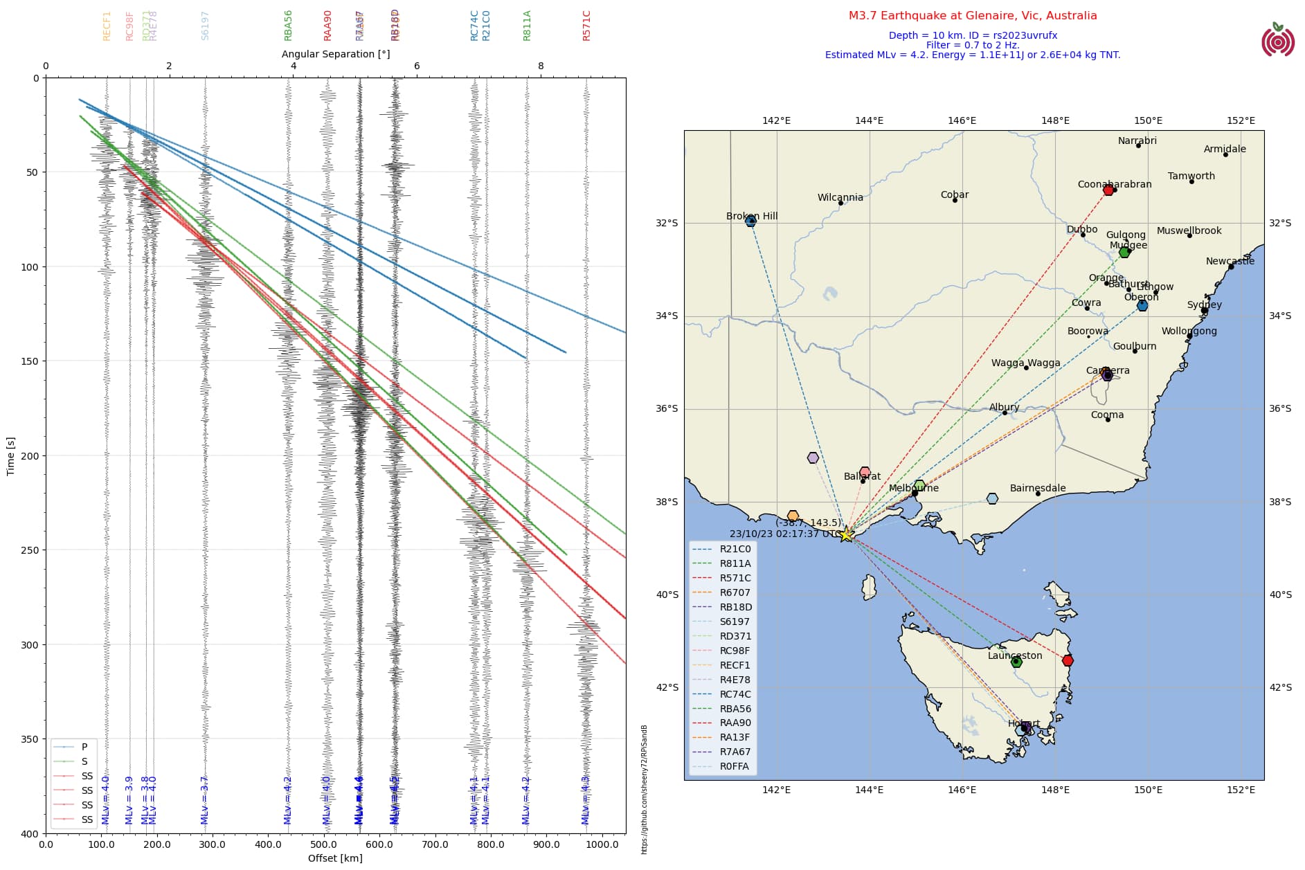
# Enter event data (estimate by trial and error for unregistered events)
eventTime = UTCDateTime(2023, 10, 23, 2, 17, 37) # (YYYY, m, d, H, M, S) **** Enter data****
latE = -38.7 # quake latitude + N -S **** Enter data****
lonE = 143.5 # quake longitude + E - W **** Enter data****
depth = 10 # quake depth, km **** Enter data****
mag = 3.7 # quake magnitude **** Enter data****
eventID = 'rs2023uvrufx' # ID for the event **** Enter data****
locE = "Glenaire, Vic, Australia" # location name **** Enter data****
slist = []
stationList(slist)
# bandpass filter - select to suit system noise and range of quake
#ft = [0.09, 0.1, 0.8, 0.9]
#ft = [0.29, 0.3, 0.8, 0.9]
#ft = [0.49, 0.5, 2, 2.1]
ft = [0.6, 0.7, 2, 2.1] #distant quake
#ft = [0.6, 0.7, 3, 3.1]
#ft = [0.6, 0.7, 4, 4.1]
#ft = [0.6, 0.7, 6, 6.1]
#ft = [0.6, 0.7, 8, 8.1]
#ft = [0.9, 1, 10, 10.1]
#ft = [0.69, 0.7, 10, 10.1]
#ft = [0.69, 0.7, 20, 20.1]
#ft = [2.9, 3, 20, 20.1] #use for local quakes
# Pretty paired colors. Reorder to have saturated colors first and remove
# some colors at the end. This cmap is compatible with obspy taup - credit to Mark Vanstone for this code.
cmap = get_cmap('Paired', lut=12)
colours = ['#%02x%02x%02x' % tuple(int(col * 255) for col in cmap(i)[:3]) for i in range(12)]
colours = colours[1:][::2][:-1] + colours[::2][:-1]
print(colours)
#colours = ['r', 'b', 'g', 'k', 'c', 'm', 'purple', 'orange', 'gold', 'midnightblue'] # array of colours for stations and phases
plist = ('P', 'S', 'SS') # phase list for plotting
#set up the plot
delay = 0 # for future development for longer distance quakes - leave as 0 for now!
duration = 400 #adjust duration to get detail required
start = eventTime + delay # for future development for longer distance quakes
end = start + duration # for future development for longer distance quakes
# Build the stream of traces/stations
st = Stream()
buildStream(st)
#set up the figure
fig = plt.figure(figsize=(20,14), dpi=100) # set to page size in inches
#build the section plot
ax1 = fig.add_subplot(1,2,1)
st.plot(type='section', plot_dx=100e3, recordlength=duration, time_down=True, linewidth=.3, alpha=0.8, grid_linewidth=.25, show=False, fig=fig)
# Plot customization: Add station labels to offset axis
ax = ax1.axes
transform = blended_transform_factory(ax.transData, ax.transAxes)
axt, axb = ax1.get_ylim() #get the top and bottom limits of the axes
#print(axt, axb)
j=0
mLav = 0
for t in st:
ax.text(t.stats.distance / 1e3, 1.05, t.stats.station, rotation=90,
va="bottom", ha="center", color=t.stats.colour, transform=transform, zorder=10)
ax.text(t.stats.distance / 1e3, axt-5, 'MLv = '+str(np.round(t.stats.mL,1)), rotation=90,
va="bottom", ha="center", color = 'b', zorder=10) #print ML estimates
mLav += t.stats.mL
j += 1
#calculate average ML estimate
mLav = mLav/j
#Calculate Earthquake Total Energy
qenergy = 10**(1.5*mLav+4.8)
#setup secondary x axis
secax_x1 = ax1.secondary_xaxis('top', functions = (k2d, d2k)) #secondary axis in degrees separation
secax_x1.set_xlabel('Angular Separation [°]')
secax_x1.xaxis.set_minor_locator(AutoMinorLocator(10))
#plot arrivals times
model = TauPyModel(model="iasp91")
axl, axr = ax1.get_xlim() # get the left and right limits of the section plot
if axl<0: #if axl is negative, make it zero to start the range for phase plots
axl=0
#axl = 150 # uncomment to adjust left side of section plot, kms
ax1.set_xlim(left = axl)
for j in range (int(axl), int(axr)): # plot phase arrivals every kilometre
arr = model.get_travel_times(depth, k2d(j), phase_list=plist)
n = len(arr)
for i in range(0,n):
if j == int(axr)-1:
ax.plot(j, arr[i].time, marker='o', markersize=1, color = colours[plist.index(arr[i].name) % len(colours)], alpha=0.3, label = arr[i].name)
else:
ax.plot(j, arr[i].time, marker='o', markersize=1, color = colours[plist.index(arr[i].name) % len(colours)], alpha=0.3)
# if j/50 == int(j/50): # periodically plot the phase name
# ax.text(j, arr[i].time, arr[i].name, color=colours[plist.index(arr[i].name) % len(colours)], alpha=0.5, ha='center', va='center')
j+=1
ax.legend(loc = 'best')
#plot the map
ax2 = fig.add_subplot(1,2,2, projection=ccrs.PlateCarree())
mt = -30 # latitude of top of map
mb = -44 # latitude of the bottom of the map
ml = 140 # longitude of the left side of the map
mr = 152.5 # longitude of the right side of the map
ax2.set_extent([ml,mr,mt,mb], crs=ccrs.PlateCarree())
#ax2.coastlines(resolution='110m') # use for large scale maps
#ax2.stock_img() # use for large scale maps
# Create a features
states_provinces = cfeature.NaturalEarthFeature(
category='cultural',
name='admin_1_states_provinces_lines',
scale='50m',
facecolor='none')
ax2.add_feature(cfeature.LAND)
ax2.add_feature(cfeature.OCEAN)
ax2.add_feature(cfeature.COASTLINE)
ax2.add_feature(states_provinces, edgecolor='gray')
ax2.add_feature(cfeature.LAKES, alpha=0.5)
ax2.add_feature(cfeature.RIVERS)
ax2.gridlines(draw_labels=True)
#plot event/earthquake position on map
ax2.plot(lonE, latE,
color='yellow', marker='*', markersize=20, markeredgecolor='black',
transform=ccrs.Geodetic(),
)
# print the lat, long, and event time beside the event marker
ax2.text(lonE-0.1, latE-0.05, "("+str(latE)+", "+str(lonE)+")\n"+eventTime.strftime('%d/%m/%y %H:%M:%S UTC'), ha='right')
#plot station positions on map
for tr in st:
ax2.plot(tr.stats.longitude, tr.stats.latitude,
color=tr.stats.colour, marker='H', markersize=12, markeredgecolor='black',
transform=ccrs.Geodetic(),
)
ax2.plot([tr.stats.longitude, lonE], [tr.stats.latitude, latE],
color=tr.stats.colour, linewidth=1, linestyle='--',
transform=ccrs.Geodetic(), label = tr.stats.station,
)
ax2.legend()
#plot places
for pl in places:
ax2.plot(pl[2], pl[1], color='k', marker='o', markersize=pl[3], markeredgecolor='k', transform=ccrs.Geodetic(), label=pl[0])
ax2.text(pl[2], pl[1]+0.05, pl[0], horizontalalignment='center', transform=ccrs.Geodetic())
#add Notes
fig.text(0.75, 0.96, 'M'+str(mag)+' Earthquake at '+locE, ha='center', size = 'large', color='r') # use for identified earthquakes
#fig.text(0.75, 0.96, 'Likely Mine Blast at '+locE, ha='center', size = 'large', color='r') # use for unidentified events
fig.text(0.75, 0.94, 'Depth = '+str(depth)+' km. ID = '+eventID, ha='center', color = 'b')
fig.text(0.75, 0.93, 'Filter = '+str(ft[1])+' to '+str(ft[2])+' Hz.', ha='center', color = 'b')
fig.text(0.75, 0.92, 'Estimated MLv = '+str(np.round(mLav,1))+'. Energy = '+f"{qenergy:0.1E}"+'J or '+f"{qenergy/4.18e6:0.1E}"+' kg TNT.', ha='center', color = 'b')
# add github repository address for code
fig.text(0.51, 0.1,'https://github.com/sheeny72/RPiSandB', size='x-small', rotation=90)
# plot logos
rsl = plt.imread("RS logo.png")
newaxr = fig.add_axes([0.935, 0.915, 0.05, 0.05], anchor='NE', zorder=-1)
newaxr.imshow(rsl)
newaxr.axis('off')
plt.subplots_adjust(wspace=0.1)
# add a plt.savefig(filename) line here if required.
plt.show()
2 Likes
Matt,
OK I’ve done some playing about. I copied your code and added enough to get it going…
The error is coming from the get_waveforms command. In the get_waveforms function change stn to stn.code. That’ll get rid of the too much data error, but will probably create a heap more as you’ll need to handle the stations that don’t have data.
I wasn’t sure how the data would be organised inside invs (i.e. whether another array layer would be added to separate the inventory for each station or not) so I put in a print(invs) line after invs is defined. It turns out invs has a lot of data in it see below.
from obspy.clients.fdsn import Client
from obspy.core import UTCDateTime, Stream

rs = Client('https://data.raspberryshake.org/')

lat = -33
lon = 150
start = UTCDateTime(2023, 10, 23, 2, 17, 0)
end = UTCDateTime(2023, 10, 23, 2, 18, 0)

invs = rs.get_stations(network='AM', latitude=lat, longitude=lon, maxradius=2, level='RESP')
stns = invs[0].stations
print(invs)
channels = ['*HZ']

stream = Stream()
for stn in stns:
    print(stn.code)
    for ch in channels:
        trace = rs.get_waveforms('AM', stn.code, '00', ch, start, end)
        stream += trace
Here’s the console output:
runfile('D:/Documents/Python/Matt Test.py', wdir='D:/Documents/Python')
Inventory created at 2023-10-23T08:57:05.375162Z
	Sending institution: SeisComP (RaspberryShake)
	Contains:
		Networks (1):
			AM
		Stations (100):
			AM.R156D (Raspberry Shake Citizen Science Station) (3x)
			AM.R21C0 (Raspberry Shake Citizen Science Station) (3x)
			AM.R2556 (Raspberry Shake Citizen Science Station)
			AM.R271A (Raspberry Shake Citizen Science Station) (3x)
			AM.R2964 (Raspberry Shake Citizen Science Station) (3x)
			AM.R2AAD (Raspberry Shake Citizen Science Station)
			AM.R2F2F (Raspberry Shake Citizen Science Station)
			AM.R3051 (Raspberry Shake Citizen Science Station)
			AM.R3756 (Raspberry Shake Citizen Science Station) (5x)
			AM.R3B68 (Raspberry Shake Citizen Science Station) (3x)
			AM.R4839 (Raspberry Shake Citizen Science Station)
			AM.R571C (Raspberry Shake Citizen Science Station) (3x)
			AM.R69A2 (Raspberry Shake Citizen Science Station)
			AM.R6EBB (Raspberry Shake Citizen Science Station) (2x)
			AM.R7AF5 (Raspberry Shake Citizen Science Station)
			AM.R7FF8 (Raspberry Shake Citizen Science Station) (2x)
			AM.R811A (Raspberry Shake Citizen Science Station) (2x)
			AM.R869F (Raspberry Shake Citizen Science Station)
			AM.R8A4D (Raspberry Shake Citizen Science Station) (4x)
			AM.R8C2E (Raspberry Shake Citizen Science Station) (5x)
			AM.R9475 (Raspberry Shake Citizen Science Station) (7x)
			AM.R965B (Raspberry Shake Citizen Science Station) (16x)
			AM.R9AF3 (Raspberry Shake Citizen Science Station) (7x)
			AM.RA656 (Raspberry Shake Citizen Science Station) (3x)
			AM.RCCE6 (Raspberry Shake Citizen Science Station) (13x)
			AM.RD2D7 (Raspberry Shake Citizen Science Station)
			AM.RE900 (Raspberry Shake Citizen Science Station)
			AM.RFB3C (Raspberry Shake Citizen Science Station) (2x)
			AM.RFD42 (Raspberry Shake Citizen Science Station)
			AM.RFE59 (Raspberry Shake Citizen Science Station)
			AM.S55E0 (Raspberry Shake Citizen Science Station) (2x)
		Channels (183):
			AM.R156D.00.SHZ (3x), AM.R21C0.00.EHZ (3x), AM.R21C0.00.HDF (3x),
			AM.R2556.00.SHZ, AM.R271A.00.EHZ (3x), AM.R271A.00.EHN (3x),
			AM.R271A.00.EHE (3x), AM.R2964.00.SHZ (3x), AM.R2AAD.00.EHZ,
			AM.R2AAD.00.HDF, AM.R2F2F.00.SHZ, AM.R3051.00.SHZ,
			AM.R3756.00.SHZ (5x), AM.R3B68.00.EHZ (3x), AM.R3B68.00.ENZ (3x),
			AM.R3B68.00.ENN (3x), AM.R3B68.00.ENE (3x), AM.R4839.00.SHZ,
			AM.R571C.00.EHZ (3x), AM.R571C.00.HDF (3x), AM.R69A2.00.SHZ,
			AM.R6EBB.00.EHZ (2x), AM.R6EBB.00.EHN (2x), AM.R6EBB.00.EHE (2x),
			AM.R7AF5.00.EHZ, AM.R7FF8.00.EHZ (2x), AM.R7FF8.00.HDF (2x),
			AM.R811A.00.EHZ (2x), AM.R869F.00.SHZ, AM.R8A4D.00.EHZ (4x),
			AM.R8A4D.00.ENZ (4x), AM.R8A4D.00.ENN (4x), AM.R8A4D.00.ENE (4x),
			AM.R8C2E.00.EHZ (5x), AM.R9475.00.SHZ (7x), AM.R965B.00.EHZ (16x),
			AM.R9AF3.00.EHZ (7x), AM.RA656.00.EHZ (3x), AM.RA656.00.ENZ (3x),
			AM.RA656.00.ENN (3x), AM.RA656.00.ENE (3x), AM.RCCE6.00.EHZ (13x),
			AM.RCCE6.00.EHN (13x), AM.RCCE6.00.EHE (13x), AM.RD2D7.00.EHZ,
			AM.RE900.00.EHZ, AM.RE900.00.ENZ, AM.RE900.00.ENN, AM.RE900.00.ENE
			AM.RFB3C.00.EHZ (2x), AM.RFB3C.00.HDF (2x), AM.RFD42.00.EHZ,
			AM.RFE59.00.EHZ, AM.RFE59.00.ENZ, AM.RFE59.00.ENN, AM.RFE59.00.ENE
			AM.S55E0.00.EHZ (2x)
R2556
Traceback (most recent call last):

  File ~\anaconda3\envs\ObspyCartopy\lib\site-packages\spyder_kernels\py3compat.py:356 in compat_exec
    exec(code, globals, locals)

  File d:\documents\python\matt test.py:20
    trace = rs.get_waveforms('AM', stn.code, '00', ch, start, end)

  File ~\anaconda3\envs\ObspyCartopy\lib\site-packages\obspy\clients\fdsn\client.py:872 in get_waveforms
    data_stream = self._download(url, use_gzip=False)

  File ~\anaconda3\envs\ObspyCartopy\lib\site-packages\obspy\clients\fdsn\client.py:1486 in _download
    raise_on_error(code, data)

  File ~\anaconda3\envs\ObspyCartopy\lib\site-packages\obspy\clients\fdsn\client.py:1813 in raise_on_error
    raise FDSNNoDataException("No data available for request.",

FDSNNoDataException: No data available for request.
HTTP Status code: 204
Detailed response of server:
That’s a lot of channels to deal with!
Al.
2 Likes
This has evolved into quite an interesting topic; keep it going!
Graibeard, welcome to our community! It’s always great to have new voices here.
1 Like
Thanks for the help, I figured out to use stn.code instead while trying to work it into a section of your code but I had no luck, I then tried it on my original one and it works but when I check for waveforms it checks the same station multiple times for whatever reason so I’ll have to figure that out.
import matplotlib.pyplot as plt

from obspy.clients.fdsn import Client
from obspy.core import UTCDateTime, Stream
from obspy.geodetics import gps2dist_azimuth

origin_time = UTCDateTime(2023, 10, 21, 15, 11, 7) # Y M D H M S
lat = -38.69
lon = 143.51

start = origin_time
end = origin_time + 1 * 60

rs = Client('RASPISHAKE')

invs = rs.get_stations(network='AM', latitude=lat, longitude=lon, maxradius=1.5, level='RESP')
stns = invs[0].stations
channels = ['EHZ']

stream = Stream()
for stn in stns:
    print(stn.code)
    try:
        for ch in channels:
            trace = rs.get_waveforms('AM', stn.code, '00', ch, start, end)
            stream += trace
            print('Data found')
    except:
        print('No data')

stream.plot()
The output is:
RDDC7
Data found
RDDC7
Data found
RDDC7
Data found
R7EE4
No data
R7EE4
No data
R9E5E
No data
RBCDA
No data
RBCDA
No data
RBCDA
No data
RBCDA
No data
RBCDA
No data
RE98F
No data
RE98F
No data
RE98F
No data
RE98F
No data
RC98F
Data found
RC98F
Data found
RDDC7
Data found
RDDC7
Data found
RDDC7
Data found
RDDC7
Data found
RDDC7
Data found
RC98F
Data found
RDDC7
Data found
RBDA2
No data
RBDA2
No data
R700E
No data
RBDA2
No data
RBDA2
No data
R700E
No data
RBDA2
No data
RBDA2
No data
RBDA2
No data
RECF1
Data found
RDDC7
Data found
And the stream plot
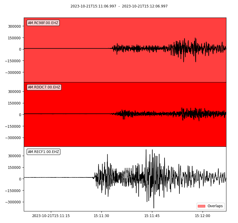
2 Likes
This is the code I use to pick up the relevant epoch from each station/channel:
 #read each epoch to find the one that's active for the event
        k=0
        while True:
            sta = inv[0][k]         #station metadata
            if sta.is_active(time=eventTime):
                break
            k += 1
For my station (R21C0), for example, there are 3 epochs: when I first set it up in the house, when I tried it in the observatory and when I moved it back to the house again. Slightly different lat longs for each epoch. So you need to find the epoch that is active at the time of the event.
Al.
3 Likes
Is that also the reason for the same station being picked up multiple times?
1 Like
Yep.
lol! this is just making up the required 20 characters for a post…
Al.
1 Like
Just a suggestion for a little tweak, Matt…
ATM your code is looking for channel ‘EHZ’. Some stations have ‘SHZ’ for the geophone channel, which might explain why you have a lot of ‘No Data’ in your above test code.
From the reading I’ve done I think you could use ‘EHZ, SHZ’ to pick up either, but I have found that ‘*HZ’ works, so I’ve been doing that to get both EHZ and SHZ channels.
Al.
2 Likes
Just been messing around at it in school and I’ve got the data collection working, thanks for the help!
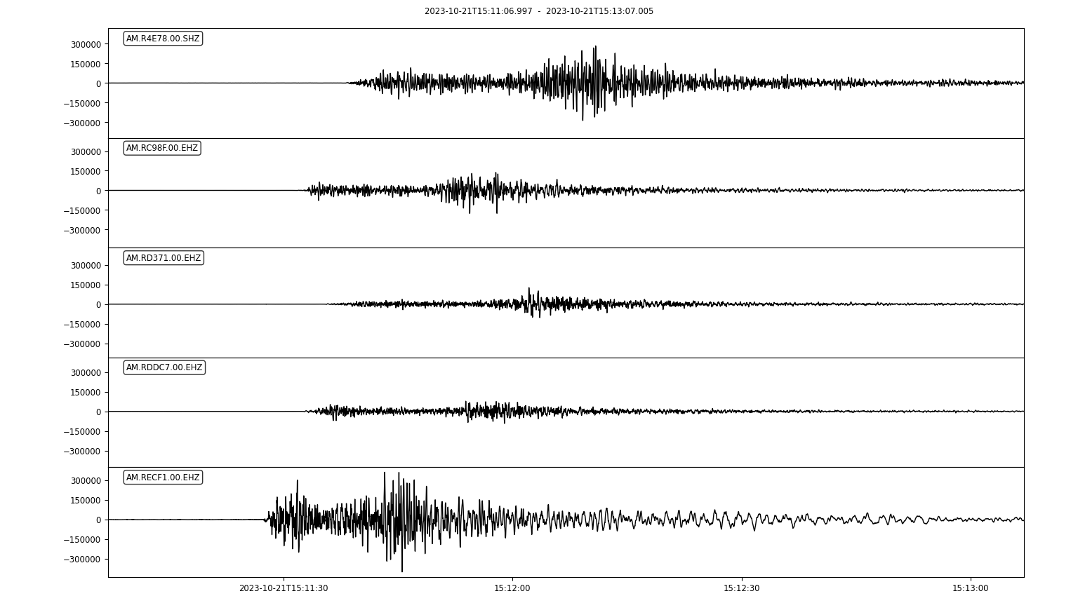
Code:
import matplotlib.pyplot as plt

from obspy.clients.fdsn import Client
from obspy.core import UTCDateTime, Stream
from obspy.geodetics import gps2dist_azimuth

origin_time = UTCDateTime(2023, 10, 21, 15, 11, 7) # Y M D H M S
latE = -38.69
lonE = 143.51

start = origin_time
end = origin_time + 2 * 60

rs = Client('RASPISHAKE')

invs = rs.get_stations(network='AM', latitude=latE, longitude=lonE, maxradius=2, level='RESP')
stns = invs[0].stations

channels = ['*HZ']

stream = Stream()
for stn in stns:
    if stn.is_active(time=start):
        print(f'Found data for {stn.code}')
        try:
            for ch in channels:
                trace = rs.get_waveforms('AM', stn.code, '00', ch, start, end)
                trace.merge(method=0, fill_value='full')
                trace.detrend(type='demean')
                stream += trace
        except:
            print(f'No data for {stn.code}')

stream.plot()
3 Likes
No worries, Matt.
Looks good!
Al.
3 Likes