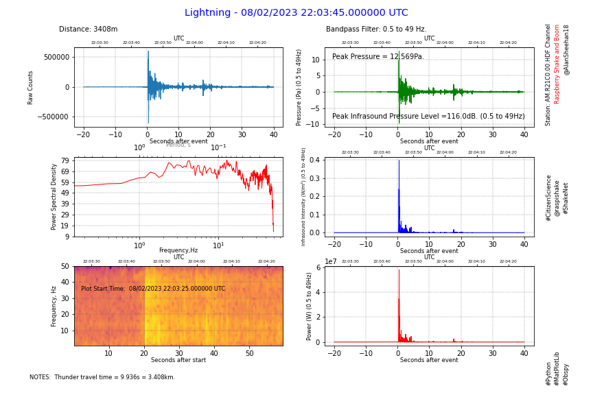
While checking and correcting Boom Event Report 2 I realised I can plot the Infrasound Intensity and calculate the point Power at the source also as traces. Boom Event Report 3 is the result. It looks like this:
And here is the code:
from obspy.clients.fdsn import Client
from obspy import UTCDateTime
import matplotlib.pyplot as plt
import numpy as np
import math

def time2UTC(a):        #convert time (seconds) since event back to UTCDateTime
    return eventTime + a

def uTC2time(a):        #convert UTCDateTime to seconds since the event
    return a - eventTime

def one_over(a):            # 1/x to convert frequency to period
    #Vectorized 1/a, treating a==0 manually
    a = np.array(a).astype(float)
    near_zero = np.isclose(a, 0)
    a[near_zero] = np.inf
    a[~near_zero] = 1 / a[~near_zero]
    return a

inverse = one_over          #function 1/x is its own inverse

def power_units(a):
    if a >= 1000000:
        return str(round(a/1000000,3))+'MW. ('
    elif a>=1000:
        return str(round(a/1000,3))+'kW. ('
    else:
        return str(round(a,3))+'W. ('

# define start and end times
eventTime = UTCDateTime(2023, 2, 8, 22, 3, 45) # (YYYY, m, d, H, M, S)
delay = -20               #delay from event time to start of plot
start = eventTime + delay   #calculate the plot start time
duration = 60               #duration of plot in seconds
end = start + duration                # start plus plot duration in seconds (recommend a minimum of 10s)

# Name the Event
eventName = 'Lightning'       # Name for the Report
distance = '3408m'          #distance to the source (use unknown if required)
notes1 = ' Thunder travel time = 9.936s = 3.408km.'  #add notes about event if desired
notes2 = ''     #add more notes if req'd
distancem = 3408                    #enter distance in metres! Enter 0 to omit.

# define fdsn client to get data from
client = Client('https://data.raspberryshake.org/')

# get data from the FSDN server and detrend it
STATION = "R21C0"               # station name
st = client.get_waveforms("AM", STATION, "00", "HDF", starttime=start, endtime=end, attach_response=True)
st.merge(method=0, fill_value='latest')
st.detrend(type="demean")

# get Instrument Response
inv = client.get_stations(network="AM", station=STATION, level="RESP")

# set-up figure and subplots
fig = plt.figure(figsize=(12,8))    #12 x 8 inches
ax1 = fig.add_subplot(6,2,(1,3))    #left top 2 high
ax2 = fig.add_subplot(6,2,(5,7))    #left middle 2 high
ax3 = fig.add_subplot(6,2,(2,4))    #right top 2 high
ax4 = fig.add_subplot(6,2,(6,8))    #right middle 2 high
ax5 = fig.add_subplot(6,2,(9,11))   #left bottom 2 high
if distancem > 0:
    ax6 = fig.add_subplot(6,2, (10, 12))    #right bottom 2 high
fig.suptitle(eventName+' - '+eventTime.strftime('%d/%m/%Y %H:%M:%S.%f UTC'), size='x-large',color='b')
fig.text(0.1, 0.92, 'Distance: '+distance)
fig.text(0.05, 0.04, 'NOTES: '+notes1, size='small')
fig.text(0.05, 0.025, notes2, size='small')
fig.text(0.92, 0.94, 'Station: AM.'+STATION+'.00.HDF Channel', size='small', rotation=90, va='top')
fig.text(0.935, 0.94, 'Raspberry Shake and Boom', size='small', rotation=90, va='top', color='r')
fig.text(0.95, 0.94, '@AlanSheehan18', size='small', rotation=90, va='top')
fig.text(0.92, 0.025, '#Python', size='small', rotation=90, va='bottom')
fig.text(0.935, 0.025, '#MatPlotLib', size='small', rotation=90, va='bottom')
fig.text(0.95, 0.025, '#Obspy', size='small', rotation=90, va='bottom')
fig.text(0.92, 0.5, '#CitizenScience', size='small', rotation=90, va='center')
fig.text(0.935, 0.5, '@raspishake', size='small', rotation=90, va='center')
fig.text(0.95, 0.5, '#ShakeNet', size='small', rotation=90, va='center')

# plot the raw curve
ax1.plot(st[0].times(reftime=eventTime), st[0].data, lw=1)

#plot the PSD
ax2.psd(x=st[0], NFFT=512, noverlap=2, Fs=100, color='r', lw=1)
ax2.set_xscale('log')

#plot spectrogram
ax5.specgram(x=st[0], NFFT=64, noverlap=16, Fs=100, cmap='plasma')
#ax5.set_yscale('log')
ax5.set_ylim(0.5,50)

# set up filter
filt = [0.5, 0.5, 49, 50]   #edit filter values to suit

# record filter settings
fig.text(0.55, 0.92,'Bandpass Filter: '+str(filt[1])+' to '+str(filt[2])+' Hz.')

# remove instrument response
resp_removed = st.remove_response(inventory=inv,pre_filt=filt,output="DEF", water_level=60)

# plot the filtered and corrected, and dB curves
ax3.plot(st[0].times(reftime=eventTime), resp_removed[0].data, lw=1, color='g')
ax4.plot(st[0].times(reftime=eventTime), resp_removed[0].data*resp_removed[0].data/397.2, lw=1, color = 'b')
if distancem > 0:
    ax6.plot(st[0].times(reftime=eventTime), resp_removed[0].data*resp_removed[0].data*4*math.pi*distancem*distancem/397.2, lw=1, color = 'r')

#calculate maximum sound pressure level
pmax = abs(resp_removed[0].max())   #find the max pressure amplitude
print(pmax)
splmax = 10*math.log10(pmax*pmax) + 93.979400087        #convert to sound pressure level
print(splmax)

#plot secondary axes - set time interval (dt) based on the duration to avoid crowding
if duration <= 9:
    dt=1           #1 seconds
elif duration <= 18:
    dt=2           #2 seconds
elif duration <= 45:
    dt=5           #5 seconds
elif duration <= 90:
    dt=10           #10 seconds
elif duration <= 180:
    dt=20          #20 seconds
elif duration <= 270:
    dt=30          #30 seconds
elif duration <= 540:
    dt=60           #1 minute
elif duration <= 1080:
    dt=120          #2 minutes
else:
    dt=300          #5 minutes
tbase = start - start.second +(int(start.second/dt)+1)*dt       #find the first time tick
tlabels = []            #initialise a blank array of time labels
tticks = []             #initialise a blank array of time ticks
sticks = []           #initialise a blank array for spectrogram ticks
nticks = int(duration/dt)+1       #calculate the number of ticks
for k in range (0, nticks):
    if dt >= 60:                #build the array of time labels - include UTC to eliminate the axis label
        tlabels.append((tbase+k*dt).strftime('%H:%M'))      #drop the seconds if not required for readability
    else:
        tlabels.append((tbase+k*dt).strftime('%H:%M:%S'))    #include seconds where required
    tticks.append(uTC2time(tbase+k*dt))                         #build the array of time ticks
    sticks.append(uTC2time(tbase+k*dt)-delay)                   #build the array of time ticks for the spectrogram
print(tlabels)                  #print the time labels - just a check for development
print(tticks)                   #print the time ticks - just a  check for development
secax_x1 = ax1.secondary_xaxis('top')       #Raw counts secondary axis
secax_x1.set_xticks(ticks=tticks)
secax_x1.set_xticklabels(tlabels, size='xx-small', va='center_baseline')
secax_x1.set_xlabel('UTC', size='small', labelpad=1)
secax_x2 = ax2.secondary_xaxis('top', functions=(one_over, inverse))        #PSD secondary axis
secax_x2.set_xlabel('Period, s', size='small', alpha=0.5, labelpad=-6)
secax_x3 = ax3.secondary_xaxis('top')       #Pascals secondary axis
secax_x3.set_xticks(ticks=tticks)
secax_x3.set_xticklabels(tlabels, size='xx-small', va='center_baseline')
secax_x3.set_xlabel('UTC', size='small', labelpad=1)
secax_x4 = ax4.secondary_xaxis('top')       #Pascals secondary axis
secax_x4.set_xticks(ticks=tticks)
secax_x4.set_xticklabels(tlabels, size='xx-small', va='center_baseline')
secax_x4.set_xlabel('UTC', size='small', labelpad=1)
secax_x5 = ax5.secondary_xaxis('top')       #Spectrogram secondary axis
secax_x5.set_xticks(ticks=sticks)
secax_x5.set_xticklabels(tlabels, size='xx-small', va='center_baseline')
secax_x5.set_xlabel('UTC', size='small', labelpad=1)
if distancem>0:
    secax_x6 = ax6.secondary_xaxis('top')       #Pascals secondary axis
    secax_x6.set_xticks(ticks=tticks)
    secax_x6.set_xticklabels(tlabels, size='xx-small', va='center_baseline')
    secax_x6.set_xlabel('UTC', size='small', labelpad=1)

# set-up some plot details
ax1.set_ylabel("Raw Counts", size='small')
ax2.set_ylabel("Power Spectral Density", size='small')
ax2.set_xlabel('Frequency,Hz', size='small',labelpad=-4)
ax3.set_ylabel("Pressure (Pa) ("+str(filt[1])+" to "+str(filt[2])+"Hz)", size='small')
ax4.set_ylabel("Infrasound Intensity (W/m²) ("+str(filt[1])+" to "+str(filt[2])+"Hz)", size='x-small')
ax5.set_ylabel("Frequency, Hz", size='small')
if distancem >0:
    ax6.set_ylabel("Power (W) ("+str(filt[1])+" to "+str(filt[2])+"Hz)", size='small')
ax1.set_xlabel("Seconds after event", size='small', labelpad=0)
ax3.set_xlabel("Seconds after event", size='small', labelpad=0)
ax4.set_xlabel("Seconds after event", size='small', labelpad=0)
ax5.set_xlabel("Seconds after start", size='small', labelpad=0)
if distancem>0:
    ax6.set_xlabel("Seconds after event", size='small', labelpad=0)

ax1.grid(color='dimgray', ls = '-.', lw = 0.33)
ax2.grid(color='dimgray', ls = '-.', lw = 0.33)
ax3.grid(color='dimgray', ls = '-.', lw = 0.33)
ax4.grid(color='dimgray', ls = '-.', lw = 0.33)
ax5.grid(color='dimgray', ls = '-.', lw = 0.33)
if distancem>0:
    ax6.grid(color='dimgray', ls = '-.', lw = 0.33)

# Report Peak Calculated Values
fig.text(0.56, 0.85, 'Peak Pressure = '+str(round(pmax,3))+'Pa.')    #report the peak Pressure
fig.text(0.56, 0.7, 'Peak Infrasound Pressure Level ='+str(round(splmax,1))+'dB. ('+str(filt[1])+" to "+str(filt[2])+"Hz)")   #report peak sound pressure level

# get the limits of the y axis so text can be consistently placed
ax5b, ax5t = ax5.get_ylim()
ax5.text(2, ax5t*0.7, 'Plot Start Time: '+start.strftime(' %d/%m/%Y %H:%M:%S.%f UTC '), size='small')      # explain difference in x time scale

#adjust subplots for readability
plt.subplots_adjust(hspace=1.2)

# save the final figure
#plt.savefig('D:\Pictures\Raspberry Shake and Boom\\'+eventName+STATION+' HDF '+start.strftime('%Y%m%d %H%M%S UTC'))  #comment this line out till figure is final

# show the final figure
plt.show()
If the distance to the source is unknown, enter 0 for distancem in line 43 and the Power will not be plotted.
Al.