A Tool for Analysing Background Noise

After playing around with multiple shakes doing section plots while chasing small local unregistered earthquakes and mine blasts, I found a lot of variation in what some stations can detect. For example, I might get a good signal on a station when using displacement for the output, but it’s unreadable in velocity and acceleration plots. Other times it might be acceleration that’s good but velocity and displacement aren’t.

This doesn’t just depend on the level of background noise, but also on the frequencies present in the noise and the choice of filter frequencies used.

I’ve written a python program to quantitatively measure background noise and determine what magnitude earthquakes should be detectable or not for a given station, filter frequencies and output.

Note: to compare the images, hover over the image and then click the dark bar at the bottom of the image. This will open the images so they can be readily clicked back and forth.


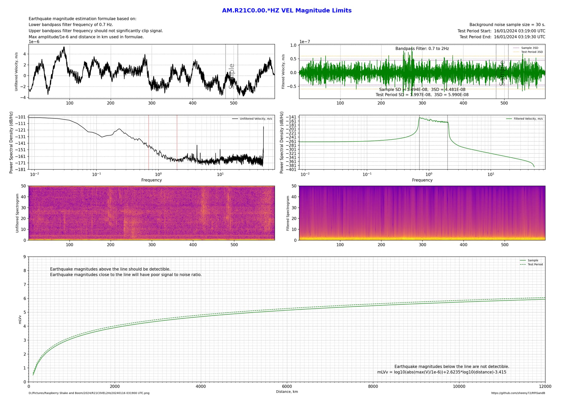
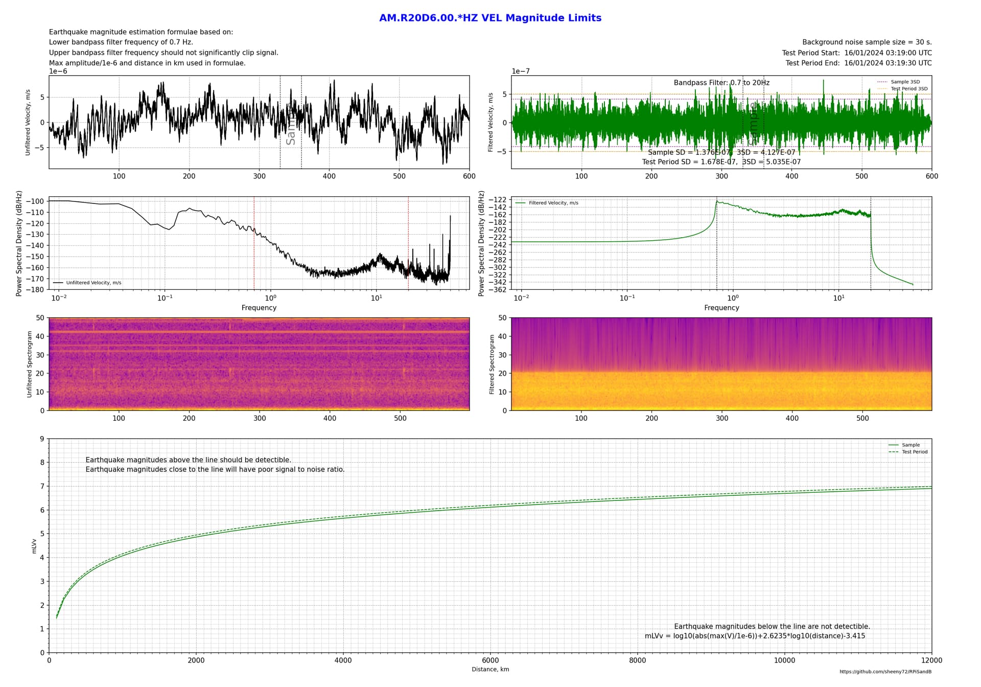
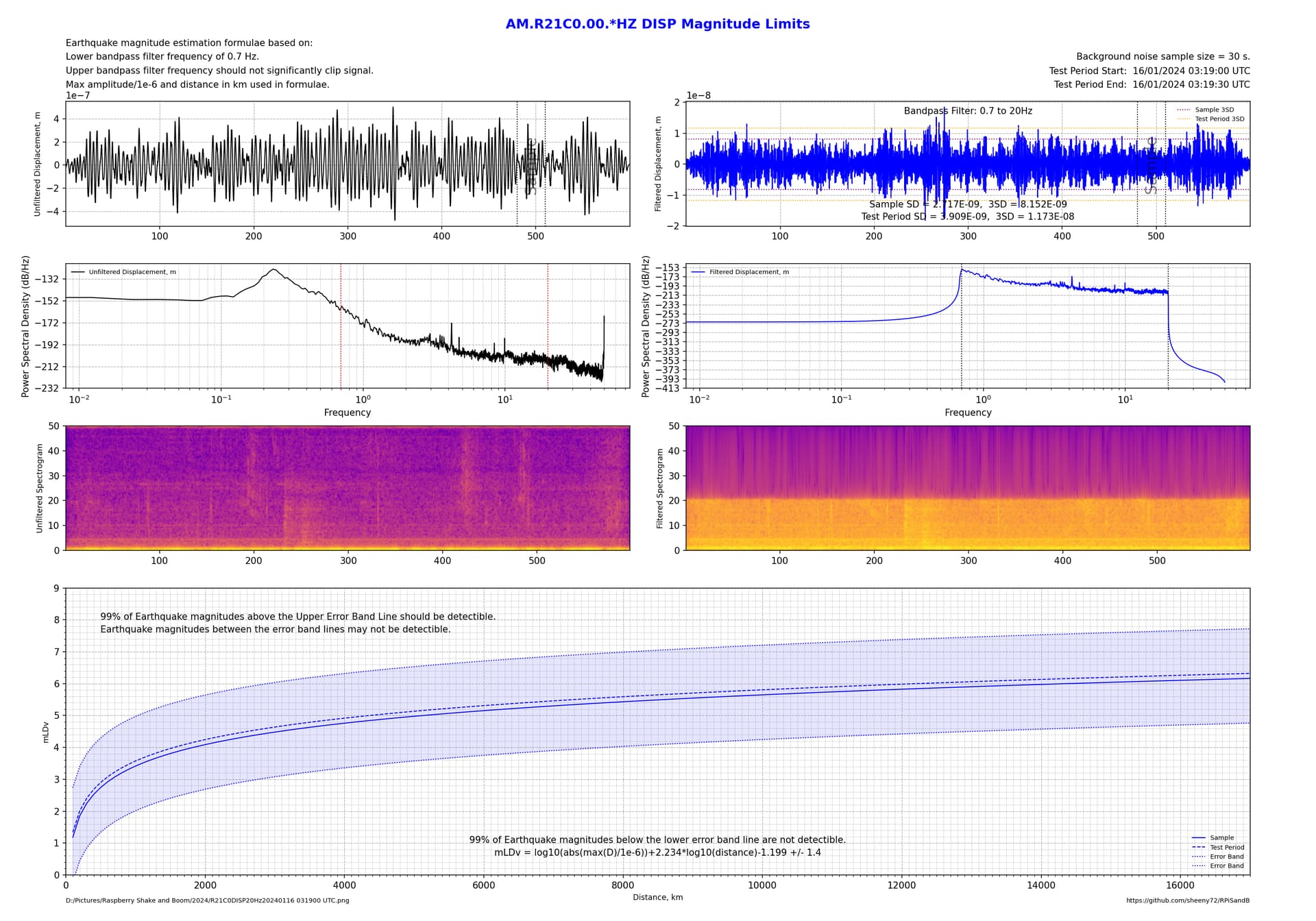
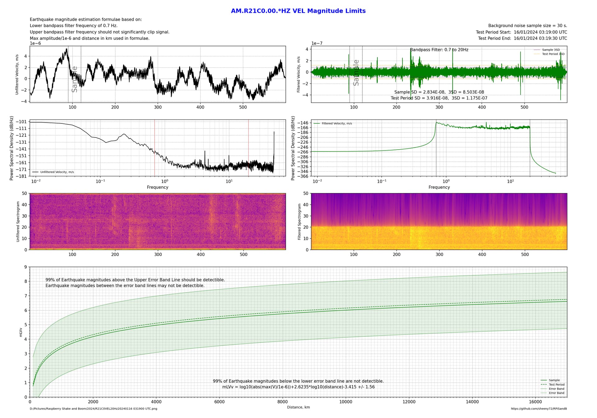
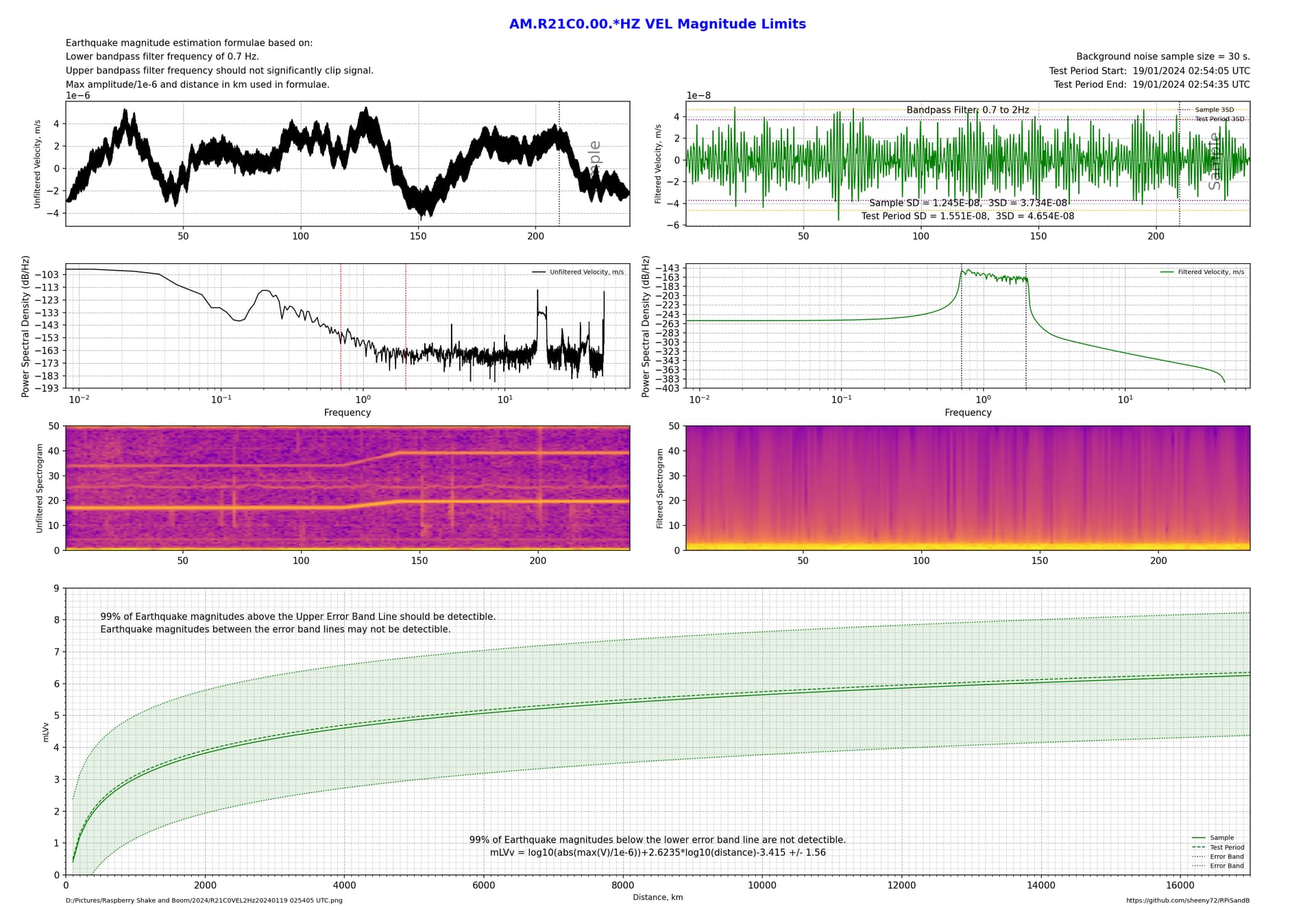
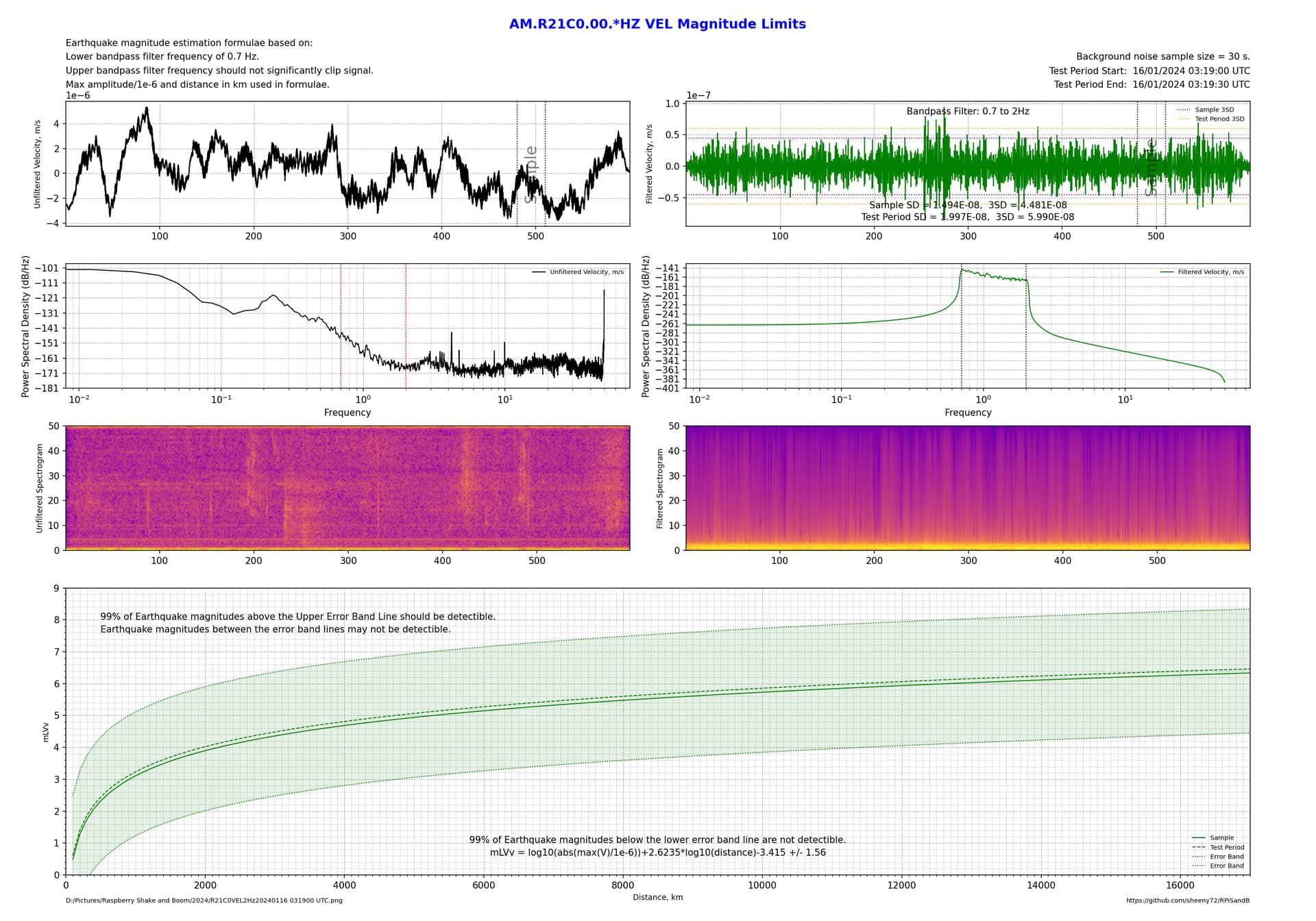
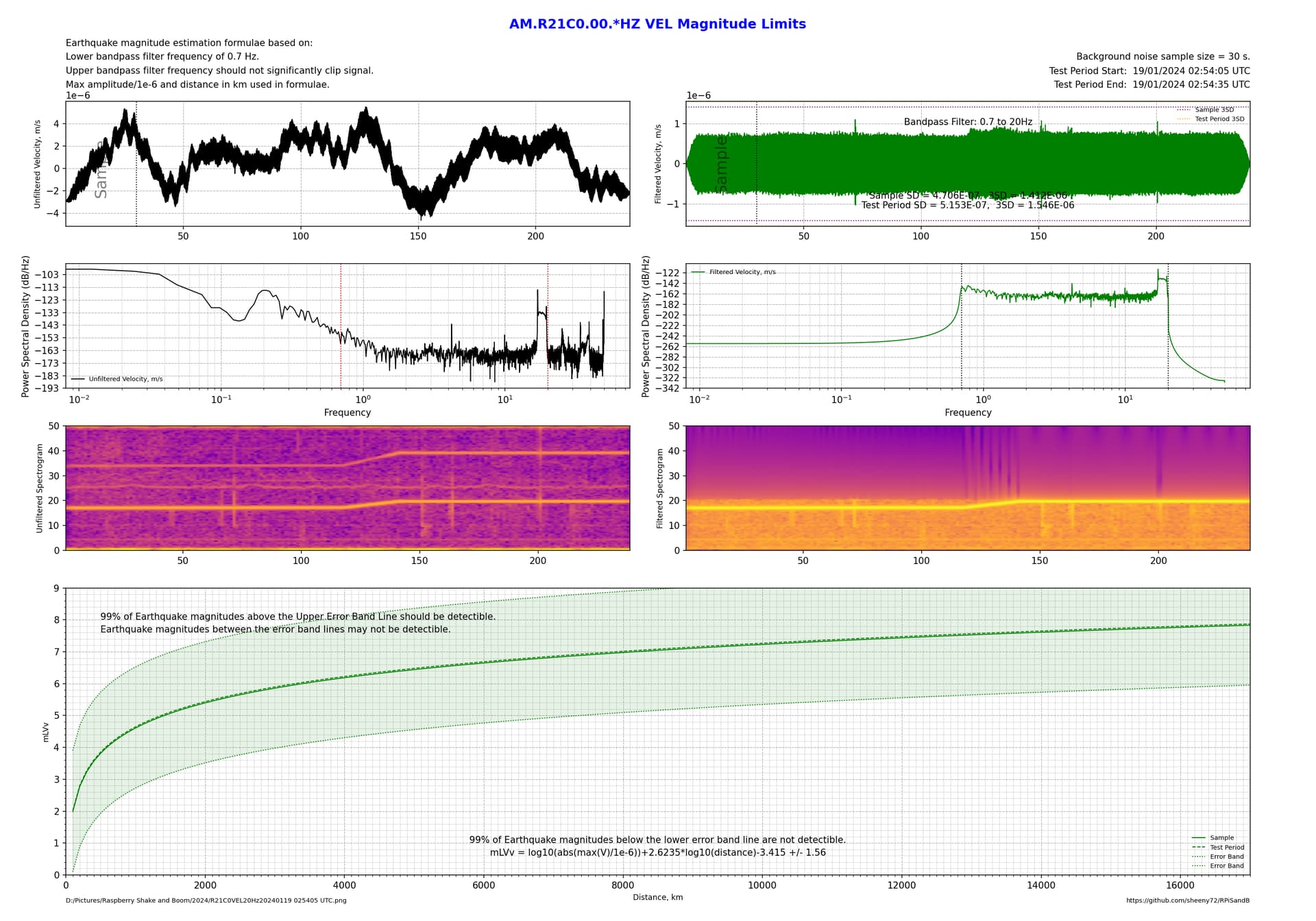
These two plots are on my station (R21C0), both at the same time, just the filter top frequency has changed. By flicking from one image to the other it can be seen that a 2Hz upper bandpass limit performs better by about 0.2 magnitudes over the whole range of distances.

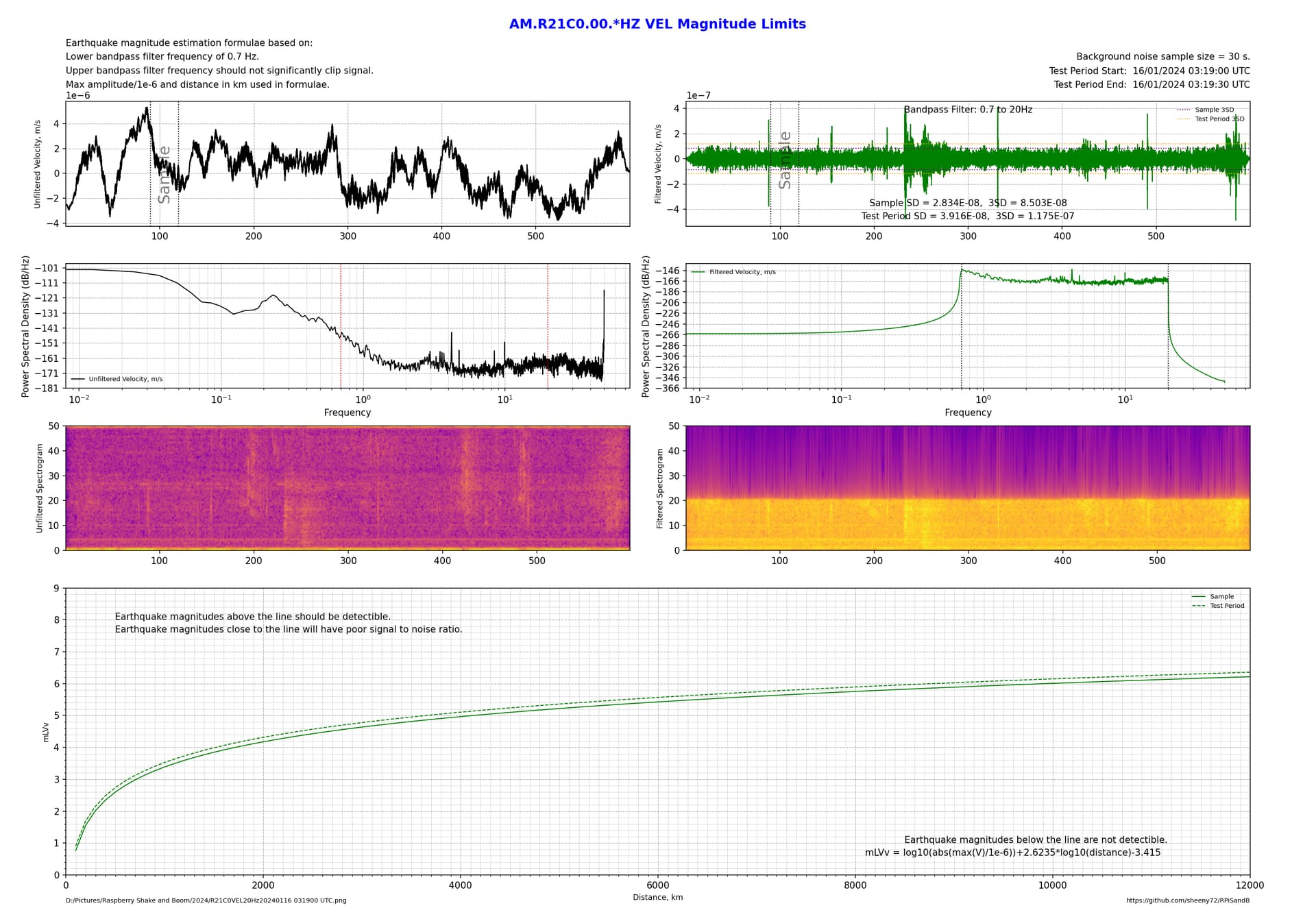
Compare this to a station installed right in the centre of Sydney:


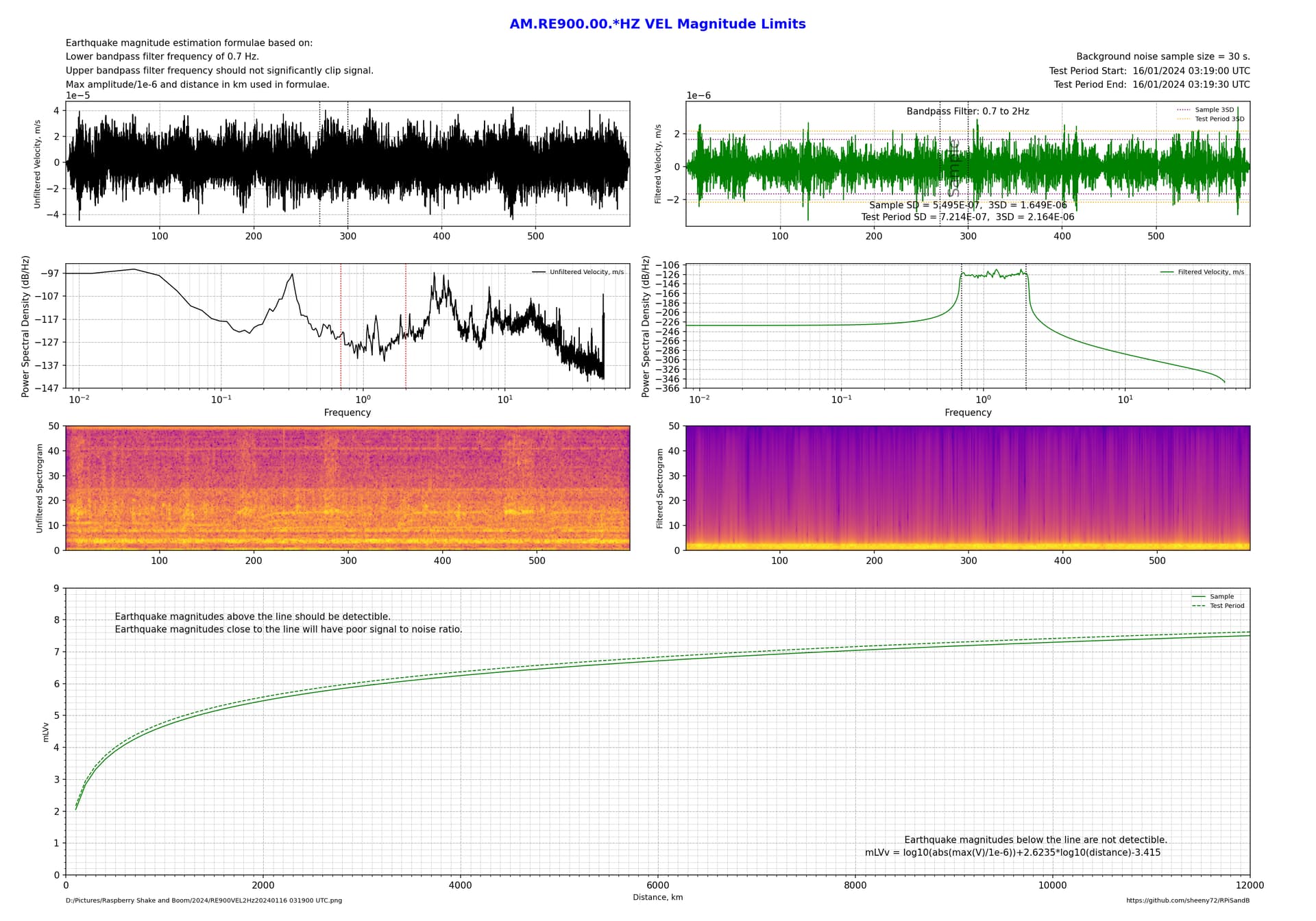
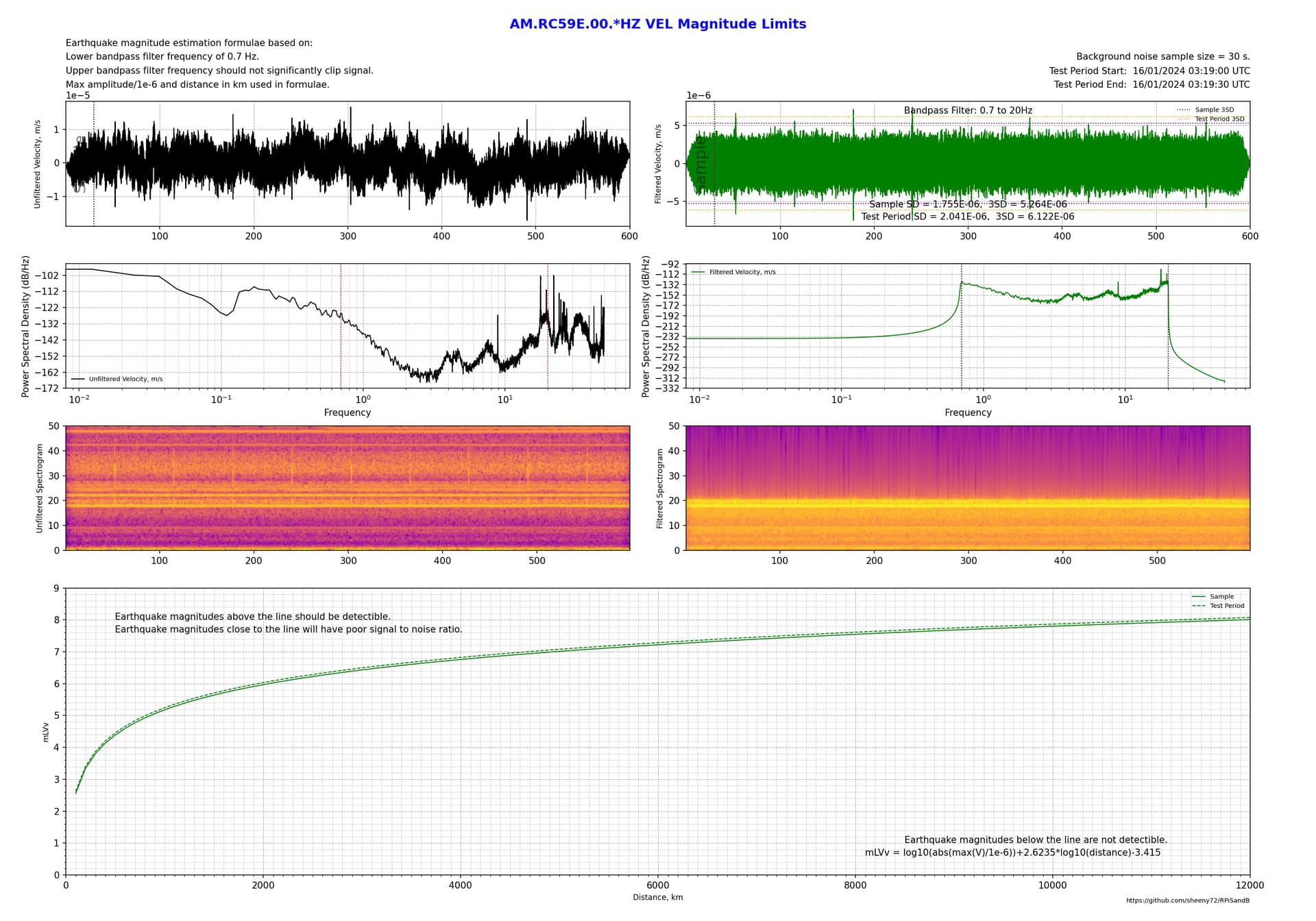
By flicking back and forth between these 2 plots shows about a 1 magnitude difference between a 2Hz upper bandpass limit and the 20Hz upper bandpass limit!

Of course, it’s also possible to compare a relatively quiet country installation with one in the city with all the additional cultural noise.

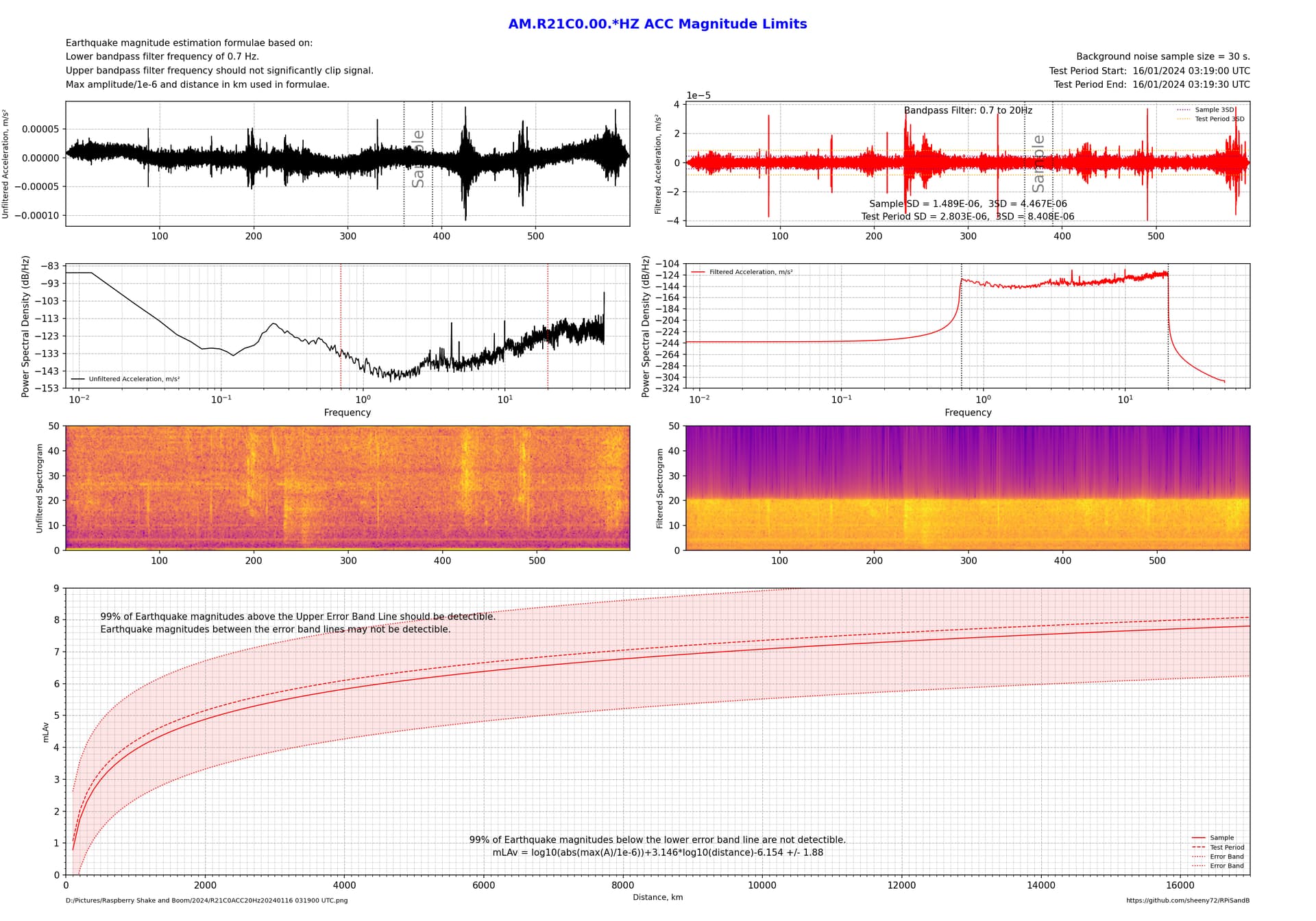
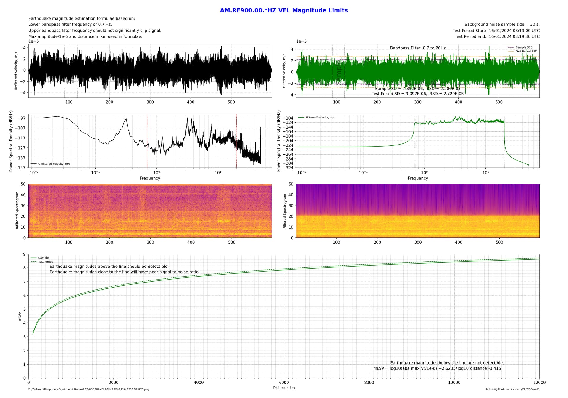
Here’s the same station in Sydney comparing Displacement, Velocity and Acceleration outputs with a maximum bandpass frequency of 20 Hz as a sort of worst case scenario:


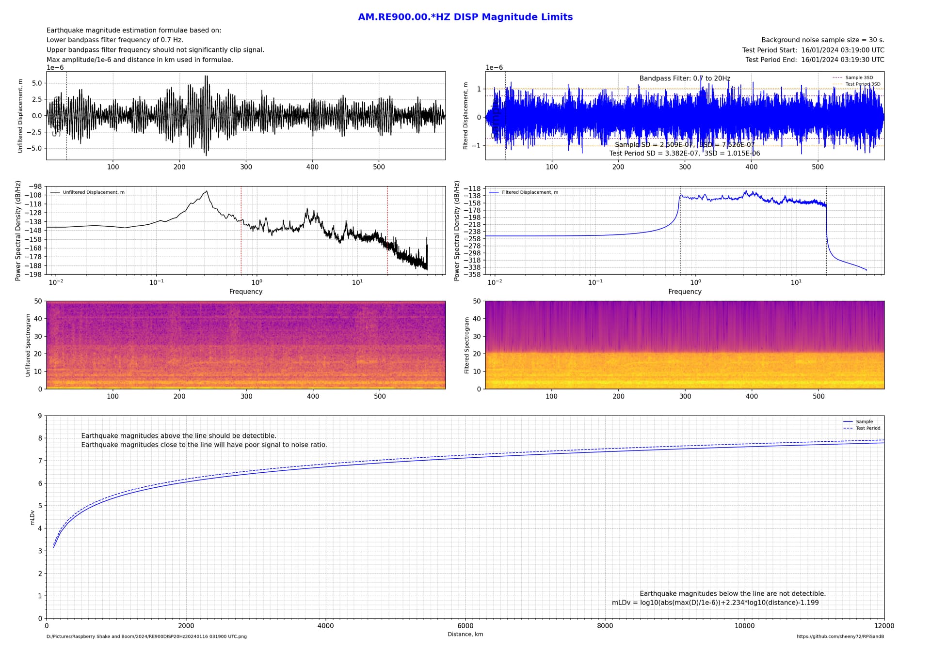
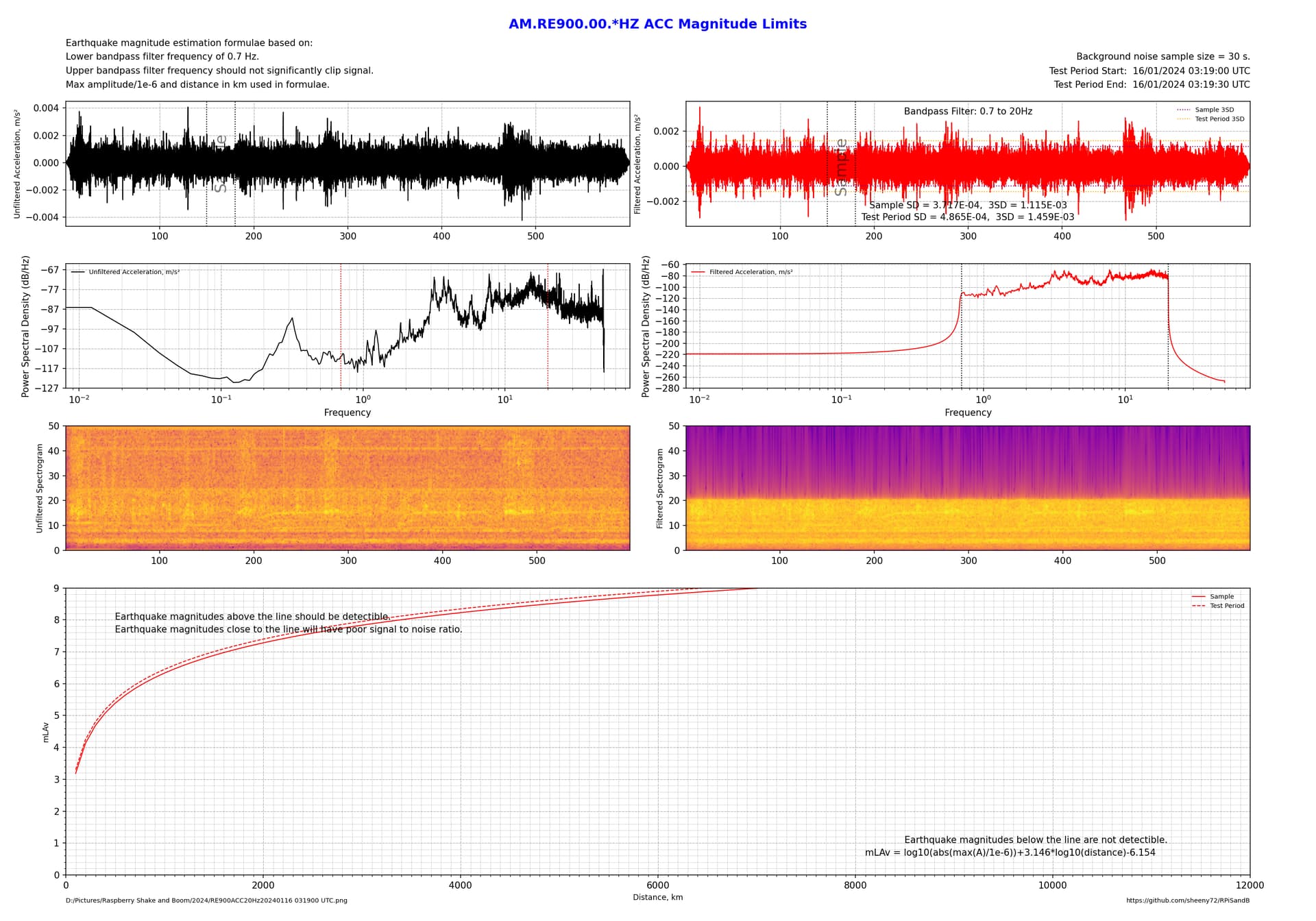
Clearly when there’s a lot of high frequency noise, apart from using a narrow bandpass filter such as 0.7 to 2 Hz, the use of Displacement also biases the lower frequencies so a better signal to noise ratio can be achieved.

This tool could also be used to quantify the effect of moving a Shake, or adding or modifying a vault, or the effect of a new noise source nearby, etc.

The code is available on Github: GitHub - sheeny72/RPiSandB: Python programs for Raspberry Shake and Boom seismometers and infrasound detectors.

I’ll share it here as well:


# -*- coding: utf-8 -*-
"""
Created on Tue Jan 16 14:56:51 2024

@author: al72

Raspberry Shake Magnitude Limits Estimator

Uses background noise measured on the Shake to estimate the minimum magnitude
earthquake detectible at any given distance.

Can be used to quantitatively compare one Shake installation and environment with another.
Can be used to compare differences in filter bands based on existing noise at the Shake.
Can be used to compare outputs (DISP v VEL v ACC) which are influenced by the
frequencies present in the background noise.

Based on magnitude estimation formulae empirically modified from the Tsuboi method
to suit 0.7 Hz lower band pass frequency for use on vertical geophone sensors on
Raspberry Shakes.

While this can be used on other sensors for comparative purposes, the accuracy of
any magnitude estimates is questionable.
"""

from obspy.clients.fdsn import Client
from obspy.core import UTCDateTime
import numpy as np
import matplotlib.pyplot as plt
from matplotlib.ticker import AutoMinorLocator
rs = Client('https://data.raspberryshake.org/')

def divTrace(tr, n):            #divide trace into n equal parts for background noise determination
    return tr.__div__(n)

def grid(ax):   #pass axis
    ax.grid(color='dimgray', ls = '-.', lw = 0.33)
    ax.grid(color='dimgray', which='minor', ls = ':', lw = 0.33)

bnstart = UTCDateTime(2024, 1, 16, 3, 19, 0) # (YYYY, m, d, H, M, S) **** Enter data****
bnend = bnstart + 600               

# set the station name and download the response information
stn = 'R21C0'      # station name
nw = 'AM'          # network name
ch = '*HZ' # ENx = accelerometer channels; EHx or SHZ = geophone channels... ONLY VALID FOR GEOPHONE CHANNELS!
#oput = 'DISP'  # output - DISP = Displacement, VEL = Velocity, ACC = Acceleration
oput = 'VEL'
#oput = 'ACC'
inv = rs.get_stations(network=nw, station=stn, level='RESP')  # get the instrument response

# bandpass filter - select to suit system noise and range of quake
filt = [0.69, 0.7, 2, 2.1]       #distant quake
#filt = [0.69, 0.7, 3, 3.1]
#filt = [0.69, 0.7, 4, 4.1]
#filt = [0.69, 0.7, 6, 6.1]
#filt = [0.69, 0.7, 8, 8.1]
#filt = [0.69, 0.7, 10, 10.1]
filt = [0.69, 0.7, 20, 20.1]
#filt = [0.69, 0.7, 49, 50]

#get waveform for background noise and copy it for independent removal of instrument response
bn0 = rs.get_waveforms('AM', stn, '00', ch, bnstart, bnend)
bn0.merge(method=0, fill_value='latest')         #fill in any gaps in the data to prevent a crash
bn0.detrend(type='demean')                       #demean the data
bn1 = bn0.copy()                                #copy for unfiltered trace

#Create background noise traces
bnfilt = bn0.remove_response(inventory=inv,pre_filt=filt,output=oput,water_level=60, plot=False) # filter the trace
bnraw = bn1.remove_response(inventory=inv,output=oput, plot=False) # unfiltered output

# Calculate background noise limits using standard deviation
bnxstd = bnfilt[0].std()            # cakculate SD for whole test period
bnsamp = 30                             #sample size in seconds
bns = int((bnend - bnstart)/bnsamp)     #calculate the number of samples in the background noise trace
bnf = divTrace(bnfilt[0],bns)           #divide the background noise trace into equal sample traces
for j in range (0, bns):                #find the sample interval with the minimum background noise amplitude
    if j == 0:
        bnfstd = abs(bnf[j].std())
        bnftime = bnf[j].stats.starttime
    elif abs(bnf[j].std()) < bnfstd:
        bnfstd = abs(bnf[j].std())
        bnftime = bnf[j].stats.starttime

mv = [] 
mLv = []
dist = []

for d in range (0,120):
    dist.append((d+1)*100)
    if oput == 'DISP':
        mLv.append(np.log10(abs(bnfstd*3/1e-6))+2.234*np.log10(dist[d])-1.199)   #calculate estimate magnitude
        mv.append(np.log10(abs(bnxstd*3/1e-6))+2.234*np.log10(dist[d])-1.199)   #calculate estimate magnitude
    elif oput == 'ACC':
        mLv.append(np.log10(abs(bnfstd*3/1e-6))+3.146*np.log10(dist[d])-6.154)   #calculate estimate magnitude
        mv.append(np.log10(abs(bnxstd*3/1e-6))+3.146*np.log10(dist[d])-6.154)   #calculate estimate magnitude
    else:
        mLv.append(np.log10(abs(bnfstd*3/1e-6))+2.6235*np.log10(dist[d])-3.415)   #calculate estimate magnitude
        mv.append(np.log10(abs(bnxstd*3/1e-6))+2.6235*np.log10(dist[d])-3.415)   #calculate estimate magnitude

if oput == 'DISP':
    colour = 'b'
    ml = 'mLDv'
    heading = 'Displacement, m'
    eq = 'mLDv = log10(abs(max(D)/1e-6))+2.234*log10(distance)-1.199'
elif oput =='ACC':
    colour = 'r'
    ml = 'mLAv'
    heading = 'Acceleration, m/s²'
    eq = 'mLAv = log10(abs(max(A)/1e-6))+3.146*log10(distance)-6.154'
else:
    colour = 'g'
    ml = 'mLVv'
    heading = 'Velocity, m/s'
    eq = 'mLVv = log10(abs(max(V)/1e-6))+2.6235*log10(distance)-3.415'
        
fig = plt.figure(figsize=(20, 14), dpi=150)       # set to page size in inches
ax1 = fig.add_subplot(5,2,1)            # raw waveform
ax2 = fig.add_subplot(5,2,2)            # filtered waveform
ax3 = fig.add_subplot(5,2,3)            # raw PSD
ax4 = fig.add_subplot(5,2,4)            # filtered PSD
ax5 = fig.add_subplot(5,2,5)            # raw spectrogram
ax6 = fig.add_subplot(5,2,6)            # spare / notes
ax7 = fig.add_subplot(5,2,(7,10))       # magnitude limit Graph

fig.suptitle(nw+'.'+stn+'.00.'+ch+' '+oput+' Magnitude Limits', weight='black', color='b', size='x-large')      #Title of the figure
ax1.plot(bn1[0].times(reftime=bnstart), bn1[0].data, lw=1, color='k')      # raw waveform
ax1.set_ylabel('Unfiltered '+heading, size='small') 
ax1.margins(x=0)
ax1.axvline(x=bnftime-bnstart, linewidth=1, linestyle='dotted', color='k')
ax1.axvline(x=(bnftime-bnstart)+bnsamp, linewidth=1, linestyle='dotted', color='k')
ax1.text(bnftime-bnstart+bnsamp/2, 0, 'Sample', size = 'xx-large', alpha = 0.5, rotation = 90, ha = 'center', va = 'center')
grid(ax1)
ax2.plot(bn1[0].times(reftime=bnstart), bn0[0].data, lw=1, color=colour)      # filtered waveform
ax2.set_ylabel('Filtered '+heading, size='small') 
ax2.margins(x=0)
ax2b, ax2t = ax2.get_ylim()
ax2.text(300, ax2t*.8, 'Bandpass Filter: '+str(filt[1])+" to "+str(filt[2])+"Hz", ha = 'center')
ax2.text(300, ax2b*0.7, 'Sample SD = '+f"{bnfstd:.3E}"+',  3SD = '+f"{(3*bnfstd):.3E}", ha = 'center')
ax2.text(300, ax2b*0.9, 'Test Period SD = '+f"{bnxstd:.3E}"+',  3SD = '+f"{(3*bnxstd):.3E}", ha = 'center')
ax2.axvline(x=bnftime-bnstart, linewidth=1, linestyle='dotted', color='k')
ax2.axvline(x=(bnftime-bnstart)+bnsamp, linewidth=1, linestyle='dotted', color='k')
ax2.text(bnftime-bnstart+bnsamp/2, 0, 'Sample', size = 'xx-large', alpha = 0.5, rotation = 90, ha = 'center', va = 'center')
ax2.axhline(y=3*bnfstd, linewidth=1, linestyle='dotted', color='purple', label = 'Sample 3SD')
ax2.axhline(y=-3*bnfstd, linewidth=1, linestyle='dotted', color='purple')
ax2.axhline(y=3*bnxstd, linewidth=1, linestyle='dotted', color='orange', label = 'Test Period 3SD')
ax2.axhline(y=-3*bnxstd, linewidth=1, linestyle='dotted', color='orange')
grid(ax2)
ax2.legend(frameon=False, fontsize='x-small', loc = 'upper right')
#plot PSD
#calculate NFFT for PSD
nfft = 8192
ax3.psd(x=bn1[0], NFFT=nfft, noverlap=0, Fs=100, color='k', lw=1, label='Unfiltered '+heading)    # velocity PSD raw data comment out if not required/desired
ax3.legend(frameon=False, fontsize='x-small')
ax3.set_xscale('log')               #use logarithmic scale on PSD
ax3.axvline(x=filt[1], linewidth=1, linestyle='dotted', color='r')
ax3.axvline(x=filt[2], linewidth=1, linestyle='dotted', color='r')
grid(ax3)
ax4.psd(x=bn0[0], NFFT=nfft, noverlap=0, Fs=100, color=colour, lw=1, label='Filtered '+heading)    # velocity PSD raw data comment out if not required/desired
ax4.legend(frameon=False, fontsize='x-small')
ax4.set_xscale('log')               #use logarithmic scale on PSD
ax4.axvline(x=filt[1], linewidth=1, linestyle='dotted', color='k')
ax4.axvline(x=filt[2], linewidth=1, linestyle='dotted', color='k')
grid(ax4)
ax5.specgram(x=bn1[0], NFFT=256, noverlap=128, Fs=100, cmap='plasma')         # raw spectrogram
ax5.set_ylabel("Unfiltered Spectrogram",size='small') 
ax6.specgram(x=bn0[0], NFFT=256, noverlap=128, Fs=100, cmap='plasma')         # raw spectrogram
ax6.set_ylabel("Filtered Spectrogram",size='small')

ax7.plot(dist, mLv, lw=1, color=colour, label = 'Sample')
ax7.plot(dist, mv, lw=1, color=colour, linestyle = '--', label = 'Test Period')
ax7.set_ylabel(ml,size='small')
ax7.set_xlabel("Distance, km",size='small')
ax7.margins(x=0)
ax7.margins(y=0)
ax7.set_ylim(0, 9)
ax7.set_xlim(0, 12000)
ax7.xaxis.set_minor_locator(AutoMinorLocator(20))
ax7.yaxis.set_minor_locator(AutoMinorLocator(5))
grid(ax7)
ax7.legend(frameon=False, fontsize='x-small')
ax7.text(500,8, 'Earthquake magnitudes above the line should be detectible.')
ax7.text(500,7.6, 'Earthquake magnitudes close to the line will have poor signal to noise ratio.')
ax7.text(8500,1, 'Earthquake magnitudes below the line are not detectible.')
ax7.text(8100,0.6, eq)

fig.text(0.05, 0.95, 'Earthquake magnitude estimation formulae based on:') 
fig.text(0.05, 0.935, 'Lower bandpass filter frequency of 0.7 Hz.')
fig.text(0.05, 0.92, 'Upper bandpass filter frequency should not significantly clip signal.')
fig.text(0.05, 0.905, 'Max amplitude/1e-6 and distance in km used in formulae.')
fig.text(0.95, 0.935, 'Background noise sample size = '+str(bnsamp)+' s.', ha = 'right')
fig.text(0.95, 0.92, 'Test Period Start: '+bnstart.strftime(' %d/%m/%Y %H:%M:%S UTC'), ha = 'right')
fig.text(0.95, 0.905, 'Test Period End: '+(bnstart+bnsamp).strftime(' %d/%m/%Y %H:%M:%S UTC'), ha = 'right')

#adjust subplots for readability
plt.subplots_adjust(hspace=0.3, wspace=0.1, left=0.05, right=0.95, bottom=0.05, top=0.89)

#print filename on bottom left corner of diagram
# Set Directory for output Plots
pics = "D:/Pictures/Raspberry Shake and Boom/2024/"      # Edit to suit **** Enter data****
filename = pics+stn+oput+str(filt[2])+'Hz'+bnstart.strftime('%Y%m%d %H%M%S UTC'+'.png')
fig.text(0.05, 0.02,filename, size='x-small')

# add github repository address for code
fig.text(0.95, 0.02,'https://github.com/sheeny72/RPiSandB', size='x-small', ha='right')

plt.savefig(filename)
# show the final figure
plt.show()
3 Likes

Super-useful sheeny! Another great work!

I couldn’t resist having a quick look at it, and I’ve plotted two VEL charts for my 3D in the quietest spot of my home (1st), and my S&B that I keep on a table nearby (2nd). Impressive (but expected) difference between base noise and earthquake detecting chances.

Will have to take a look at the other variables (DISP, ACC) and filter options. A recommended tool to explore one’s very local indoor (or outdoor) environment and find the best spot for a new Shake.

I would just add a disclaimer that (for now) this program doesn’t (yet) take into account EQ shadow zones and PKP caustics, so if EQs are not detected in the first case, or are instead detected close to the second, users are not surprised.

1 Like

Thanks Stormchaser.

Wow! About 1 magnitude! The Unfiltered PSD really shows the difference above 10Hz. A 0.7 to 2 Hz (even 3 Hz) filter looks like it would give very similar performance on both stations.

It’s also interesting to compare the difference at the very low frequency end between your station and mine.

I’m not sure how to include anything in the code to account for shadow zones, etc. It’s based purely on the algorithms for estimating the magnitude of quakes, which use the maximum amplitude regardless of the phase, so I don’t think it matters. In the shadow zone, the peak amplitude is usually a phase other than P or S and the algorithm still uses whatever is the maximum amplitude.

Al.

2 Likes

While testing the code I tried a few other local shakes which I know work both better and worse than mine (either less or more background noise) and was surprised that the difference wasn’t more in terms of magnitudes based on experience. I guess even small improvements in terms of magnitude can make a big difference to how many quakes you can detect.

Al.

2 Likes

I should make another note:

The algorithms used to estimate the quake magnitudes are subject to errors (not mistakes, but inaccuracies). This is the result of the original (official) Magnitude estimates also being subject to errors (It’s not a precise science), as well as the statistical errors from data scatter when trying to statistically derive the empirical formulae for the estimations, and variations in signal attenuation because a higher low frequency bandpass filter limit was used (0.7Hz instead of 0.033Hz) in order to lower the magnitudes that can be detectable.

For mLDv the error is +/- 1.4 magnitudes.
For mLVv the error is +/- 1.56 magnitudes.
For mLAv the erros is +/- 1.9 magnitudes.

So this means:
It is possible to detect a quake 1.56 magnitudes below the line with velocity output.
It is possible to NOT detect a quake 1.56 magnitudes above the line with velocity output.

However, for the sake of comparison of signal sensitivity based on background noise, the Limiting Magnitude Plot is valid and accurate (as it is based on the line of best fit through the original data).

I was reminded to make this comment this morning as my shake detected a M5 quake from Mariana Islands 5680 kms away. This put it just below the sample line on the Magnitude Limit plot for 0.7 to 2Hz, yet the amplitude of the initial P spike was clearly detectable. Other quakes of the same magnitude at the same distance are not detectable.

Al.

2 Likes

Yes, a full magnitude difference between the two! Amazing that I can now quantify this value with precision thanks to the program you’ve written.

I imagined that it would have been complex to integrate shadow zones and PKP caustics, but all the details that you’ve added give a definite and more rounded view of the capabilities of your code.

Do you think that it would be possible to add these +/- error margins to the initial plot in a way similar to this?

With a semi-transparent area around the principal line and adding those values in a legend? I think it would add even more precision/details to the overall program.

Also, another suggestion I had but forgot to mention, what do you think about extending the x-axis range of the last plot to reach the 15000/17000 km away from the station? In this way, we should be able to see what happens regarding long-distance events.

1 Like

Yep, good thinking.

When I wrote it I really was only thinking about a tool for comparison, not a definitive guide for what is detectable. It was only when I realised the Magnitude Limit isn’t a hard limit because of the errors I thought I’d better explain that because someone will call it out eventually.

I’ll do some polishing! ;o)

Al.

2 Likes

Revision 1:

I’ve added the error bands and increased the max distance to 17000 kms and I’ve added a duration variable so the duration of the traces can be readily adjusted.

(And now I’ve learned to fill_between) ;o)

Al.


# -*- coding: utf-8 -*-
"""
Created on Tue Jan 16 14:56:51 2024

@author: al72

Raspberry Shake Magnitude Limits Estimator

Uses background noise measured on the Shake to estimate the minimum magnitude
earthquake detectible at any given distance.

Can be used to quantitatively compare one Shake installation and environment with another.
Can be used to compare differences in filter bands based on existing noise at the Shake.
Can be used to compare outputs (DISP v VEL v ACC) which are influenced by the
frequencies present in the background noise.

Based on magnitude estimation formulae empirically modified from the Tsuboi method
to suit 0.7 Hz lower band pass frequency for use on vertical geophone sensors on
Raspberry Shakes.

While this can be used on other sensors for comparative purposes, the accuracy of
any magnitude estimates is questionable.
"""

from obspy.clients.fdsn import Client
from obspy.core import UTCDateTime
import numpy as np
import matplotlib.pyplot as plt
from matplotlib.ticker import AutoMinorLocator
rs = Client('https://data.raspberryshake.org/')

def divTrace(tr, n):            #divide trace into n equal parts for background noise determination
    return tr.__div__(n)

def grid(ax):   #pass axis
    ax.grid(color='dimgray', ls = '-.', lw = 0.33)
    ax.grid(color='dimgray', which='minor', ls = ':', lw = 0.33)

bnstart = UTCDateTime(2024, 1, 16, 3, 19, 0) # (YYYY, m, d, H, M, S) **** Enter data****
duration = 600
bnend = bnstart + duration               

# set the station name and download the response information
stn = 'R21C0'      # station name
nw = 'AM'          # network name
ch = '*HZ' # ENx = accelerometer channels; EHx or SHZ = geophone channels... ONLY VALID FOR GEOPHONE CHANNELS!
#oput = 'DISP'  # output - DISP = Displacement, VEL = Velocity, ACC = Acceleration
oput = 'VEL'
#oput = 'ACC'
inv = rs.get_stations(network=nw, station=stn, level='RESP')  # get the instrument response

# bandpass filter - select to suit system noise and range of quake
filt = [0.69, 0.7, 2, 2.1]       #distant quake
#filt = [0.69, 0.7, 3, 3.1]
#filt = [0.69, 0.7, 4, 4.1]
#filt = [0.69, 0.7, 6, 6.1]
#filt = [0.69, 0.7, 8, 8.1]
#filt = [0.69, 0.7, 10, 10.1]
#filt = [0.69, 0.7, 20, 20.1]
#filt = [0.69, 0.7, 49, 50]

#get waveform for background noise and copy it for independent removal of instrument response
bn0 = rs.get_waveforms('AM', stn, '00', ch, bnstart, bnend)
bn0.merge(method=0, fill_value='latest')         #fill in any gaps in the data to prevent a crash
bn0.detrend(type='demean')                       #demean the data
bn1 = bn0.copy()                                #copy for unfiltered trace

#Create background noise traces
bnfilt = bn0.remove_response(inventory=inv,pre_filt=filt,output=oput,water_level=60, plot=False) # filter the trace
bnraw = bn1.remove_response(inventory=inv,output=oput, plot=False) # unfiltered output

# Calculate background noise limits using standard deviation
bnxstd = bnfilt[0].std()            # cakculate SD for whole test period
bnsamp = 30                             #sample size in seconds
bns = int((bnend - bnstart)/bnsamp)     #calculate the number of samples in the background noise trace
bnf = divTrace(bnfilt[0],bns)           #divide the background noise trace into equal sample traces
for j in range (0, bns):                #find the sample interval with the minimum background noise amplitude
    if j == 0:
        bnfstd = abs(bnf[j].std())
        bnftime = bnf[j].stats.starttime
    elif abs(bnf[j].std()) < bnfstd:
        bnfstd = abs(bnf[j].std())
        bnftime = bnf[j].stats.starttime

mv = [] 
mLv = []
errh = []
errl = []
dist = []

for d in range (0,170):
    dist.append((d+1)*100)
    if oput == 'DISP':
        mLv.append(np.log10(abs(bnfstd*3/1e-6))+2.234*np.log10(dist[d])-1.199)   #calculate estimate magnitude
        mv.append(np.log10(abs(bnxstd*3/1e-6))+2.234*np.log10(dist[d])-1.199)   #calculate estimate magnitude
        errl.append(mLv[d]-1.4)
        errh.append(mv[d]+1.4)
    elif oput == 'ACC':
        mLv.append(np.log10(abs(bnfstd*3/1e-6))+3.146*np.log10(dist[d])-6.154)   #calculate estimate magnitude
        mv.append(np.log10(abs(bnxstd*3/1e-6))+3.146*np.log10(dist[d])-6.154)   #calculate estimate magnitude
        errl.append(mLv[d]-1.56)
        errh.append(mv[d]+1.56)
    else:
        mLv.append(np.log10(abs(bnfstd*3/1e-6))+2.6235*np.log10(dist[d])-3.415)   #calculate estimate magnitude
        mv.append(np.log10(abs(bnxstd*3/1e-6))+2.6235*np.log10(dist[d])-3.415)   #calculate estimate magnitude
        errl.append(mLv[d]-1.88)
        errh.append(mv[d]+1.88)

if oput == 'DISP':
    colour = 'b'
    ml = 'mLDv'
    heading = 'Displacement, m'
    eq = 'mLDv = log10(abs(max(D)/1e-6))+2.234*log10(distance)-1.199 +/- 1.4'
elif oput =='ACC':
    colour = 'r'
    ml = 'mLAv'
    heading = 'Acceleration, m/s²'
    eq = 'mLAv = log10(abs(max(A)/1e-6))+3.146*log10(distance)-6.154 +/- 1.88'
else:
    colour = 'g'
    ml = 'mLVv'
    heading = 'Velocity, m/s'
    eq = 'mLVv = log10(abs(max(V)/1e-6))+2.6235*log10(distance)-3.415 +/- 1.56'
        
fig = plt.figure(figsize=(20, 14), dpi=150)       # set to page size in inches
ax1 = fig.add_subplot(5,2,1)            # raw waveform
ax2 = fig.add_subplot(5,2,2)            # filtered waveform
ax3 = fig.add_subplot(5,2,3)            # raw PSD
ax4 = fig.add_subplot(5,2,4)            # filtered PSD
ax5 = fig.add_subplot(5,2,5)            # raw spectrogram
ax6 = fig.add_subplot(5,2,6)            # spare / notes
ax7 = fig.add_subplot(5,2,(7,10))       # magnitude limit Graph

fig.suptitle(nw+'.'+stn+'.00.'+ch+' '+oput+' Magnitude Limits', weight='black', color='b', size='x-large')      #Title of the figure
ax1.plot(bn1[0].times(reftime=bnstart), bn1[0].data, lw=1, color='k')      # raw waveform
ax1.set_ylabel('Unfiltered '+heading, size='small') 
ax1.margins(x=0)
ax1.axvline(x=bnftime-bnstart, linewidth=1, linestyle='dotted', color='k')
ax1.axvline(x=(bnftime-bnstart)+bnsamp, linewidth=1, linestyle='dotted', color='k')
ax1.text(bnftime-bnstart+bnsamp/2, 0, 'Sample', size = 'xx-large', alpha = 0.5, rotation = 90, ha = 'center', va = 'center')
grid(ax1)
ax2.plot(bn1[0].times(reftime=bnstart), bn0[0].data, lw=1, color=colour)      # filtered waveform
ax2.set_ylabel('Filtered '+heading, size='small') 
ax2.margins(x=0)
ax2b, ax2t = ax2.get_ylim()
ax2.text(duration/2, ax2t*.8, 'Bandpass Filter: '+str(filt[1])+" to "+str(filt[2])+"Hz", ha = 'center')
ax2.text(duration/2, ax2b*0.7, 'Sample SD = '+f"{bnfstd:.3E}"+',  3SD = '+f"{(3*bnfstd):.3E}", ha = 'center')
ax2.text(duration/2, ax2b*0.9, 'Test Period SD = '+f"{bnxstd:.3E}"+',  3SD = '+f"{(3*bnxstd):.3E}", ha = 'center')
ax2.axvline(x=bnftime-bnstart, linewidth=1, linestyle='dotted', color='k')
ax2.axvline(x=(bnftime-bnstart)+bnsamp, linewidth=1, linestyle='dotted', color='k')
ax2.text(bnftime-bnstart+bnsamp/2, 0, 'Sample', size = 'xx-large', alpha = 0.5, rotation = 90, ha = 'center', va = 'center')
ax2.axhline(y=3*bnfstd, linewidth=1, linestyle='dotted', color='purple', label = 'Sample 3SD')
ax2.axhline(y=-3*bnfstd, linewidth=1, linestyle='dotted', color='purple')
ax2.axhline(y=3*bnxstd, linewidth=1, linestyle='dotted', color='orange', label = 'Test Period 3SD')
ax2.axhline(y=-3*bnxstd, linewidth=1, linestyle='dotted', color='orange')
grid(ax2)
ax2.legend(frameon=False, fontsize='x-small', loc = 'upper right')
#plot PSD
#calculate NFFT for PSD
nfft = 8192
ax3.psd(x=bn1[0], NFFT=nfft, noverlap=0, Fs=100, color='k', lw=1, label='Unfiltered '+heading)    # velocity PSD raw data comment out if not required/desired
ax3.legend(frameon=False, fontsize='x-small')
ax3.set_xscale('log')               #use logarithmic scale on PSD
ax3.axvline(x=filt[1], linewidth=1, linestyle='dotted', color='r')
ax3.axvline(x=filt[2], linewidth=1, linestyle='dotted', color='r')
grid(ax3)
ax4.psd(x=bn0[0], NFFT=nfft, noverlap=0, Fs=100, color=colour, lw=1, label='Filtered '+heading)    # velocity PSD raw data comment out if not required/desired
ax4.legend(frameon=False, fontsize='x-small')
ax4.set_xscale('log')               #use logarithmic scale on PSD
ax4.axvline(x=filt[1], linewidth=1, linestyle='dotted', color='k')
ax4.axvline(x=filt[2], linewidth=1, linestyle='dotted', color='k')
grid(ax4)
ax5.specgram(x=bn1[0], NFFT=256, noverlap=128, Fs=100, cmap='plasma')         # raw spectrogram
ax5.set_ylabel("Unfiltered Spectrogram",size='small') 
ax6.specgram(x=bn0[0], NFFT=256, noverlap=128, Fs=100, cmap='plasma')         # raw spectrogram
ax6.set_ylabel("Filtered Spectrogram",size='small')

ax7.plot(dist, mLv, lw=1, color=colour, label = 'Sample')
ax7.plot(dist, mv, lw=1, color=colour, linestyle = '--', label = 'Test Period')
ax7.plot(dist, errl, lw=1, color=colour, linestyle = ':', label = 'Error Band')
ax7.plot(dist, errh, lw=1, color=colour, linestyle = ':', label = 'Error Band')
ax7.fill_between(dist, errl, errh, color=colour, alpha=0.1)
ax7.set_ylabel(ml,size='small')
ax7.set_xlabel("Distance, km",size='small')
ax7.margins(x=0)
ax7.margins(y=0)
ax7.set_ylim(0, 9)
ax7.set_xlim(0, 17000)
ax7.xaxis.set_minor_locator(AutoMinorLocator(20))
ax7.yaxis.set_minor_locator(AutoMinorLocator(5))
grid(ax7)
ax7.legend(frameon=False, fontsize='x-small', loc = 'lower right')
ax7.text(500,8, '99% of Earthquake magnitudes above the Upper Error Band Line should be detectible.')
ax7.text(500,7.6, 'Earthquake magnitudes between the error band lines may not be detectible.')
ax7.text(8500,1, '99% of Earthquake magnitudes below the lower error band line are not detectible.', ha = 'center')
ax7.text(8500,0.6, eq, ha = 'center')

fig.text(0.05, 0.95, 'Earthquake magnitude estimation formulae based on:') 
fig.text(0.05, 0.935, 'Lower bandpass filter frequency of 0.7 Hz.')
fig.text(0.05, 0.92, 'Upper bandpass filter frequency should not significantly clip signal.')
fig.text(0.05, 0.905, 'Max amplitude/1e-6 and distance in km used in formulae.')
fig.text(0.95, 0.935, 'Background noise sample size = '+str(bnsamp)+' s.', ha = 'right')
fig.text(0.95, 0.92, 'Test Period Start: '+bnstart.strftime(' %d/%m/%Y %H:%M:%S UTC'), ha = 'right')
fig.text(0.95, 0.905, 'Test Period End: '+(bnstart+bnsamp).strftime(' %d/%m/%Y %H:%M:%S UTC'), ha = 'right')

#adjust subplots for readability
plt.subplots_adjust(hspace=0.3, wspace=0.1, left=0.05, right=0.95, bottom=0.05, top=0.89)

#print filename on bottom left corner of diagram
# Set Directory for output Plots
pics = "D:/Pictures/Raspberry Shake and Boom/2024/"      # Edit to suit **** Enter data****
filename = pics+stn+oput+str(filt[2])+'Hz'+bnstart.strftime('%Y%m%d %H%M%S UTC'+'.png')
fig.text(0.05, 0.02,filename, size='x-small')

# add github repository address for code
fig.text(0.95, 0.02,'https://github.com/sheeny72/RPiSandB', size='x-small', ha='right')

plt.savefig(filename)
# show the final figure
plt.show()

2 Likes

Just for curiosity, I thought I’d see what effect the washing machine on spin cycle has on the ability to detect quakes.

Washing machine on spin cycle, 0.7 to 2Hz filter, velocity:

Reference 0.7 to 2 Hz filter, velocity:

Comparing the two, it’s pretty similar (in fact slightly better - but that’s not due to the washing machine!) so detecting distant quakes isn’t affected much at all.

Washing machine on spin cycle, 0.7 to 20Hz filter, velocity:

Reference 0.7 to 20Hz filter, velocity:

Comparing the two, there’s a 1.2 magnitude difference. I regularly use the 0.7 to 20Hz filter on local quakes and mine blasts, so the washing machine reduces the ability to detect these by 1.2 magnitudes. Given the local quakes and mine blasts are usually small in magnitude anyway (< M3.5) 1.2 magnitudes is a big deal.

Al.

2 Likes

Impressive, great work Al!

I noticed the same with my washing machine while it is doing its spinning up/down cycles, and it is interesting to see how such super-local vibrations do not affect almost at all detection of far-away earthquakes.

If I open my DataView stream and filter the trace to my usual 0.7 Hz to 2.0 Hz, there is little to no trace of those cycles, even if they appear clearly in the unfiltered spectrogram.

I hope this program will be very useful to all Shakers around the world.

1 Like